Separating Signal From Noise With ICA

Separating Signal From Noise With ICA#

Written by Luke Chang

In this tutorial we will use ICA to explore which signals in our imaging data might be real signal or artifacts. We cover ICA in more depth in the [multivariate-decomposition] subsection of the connectivity tutorial and also using simulations in the ICA tutorial.

To run this tutorial, we will be working with data that has already been preprocessed. If you are in Psych60, this has already been done for you. If you reading this online, then I recommend reading the preprocessing tutorial, or downloading the data using the datalad tutorial.

For a brief overview of types of artifacts that might be present in your data, I recommend watching this video by Tor Wager and Martin Lindquist.

from IPython.display import YouTubeVideo

YouTubeVideo('7Kk_RsGycHs')

Loading Data#

Ok, let’s load a subject and run an ICA to explore signals that are present. Since we have completed preprocessing, our data should be realigned and also normalized to MNI stereotactic space. We will use the nltools package to work with this data in python.

%matplotlib inline

import os
import glob
import numpy as np
import pandas as pd
import matplotlib.pyplot as plt
import seaborn as sns
from nltools.data import Brain_Data
from nltools.plotting import component_viewer

base_dir = '../data/localizer/derivatives/preproc/fmriprep'
base_dir = '/Users/lukechang/Dropbox/Dartbrains/Data/preproc/fmriprep'
sub = 'S01'

data = Brain_Data(os.path.join(base_dir, f'sub-{sub}','func', f'sub-{sub}_task-localizer_space-MNI152NLin2009cAsym_desc-preproc_bold.nii.gz'))

More Preprocessing#

Even though, we have technically already run most of the preprocessing there are a couple of more steps that will help make the ICA cleaner.

First, we will run a high pass filter to remove any low frequency scanner drift. We will pick a fairly arbitrary filter size of 0.0078hz (1/128s). We will also run spatial smoothing with a 6mm FWHM gaussian kernel to increase a signal to noise ratio at each voxel. These steps are very easy to run using nltools after the data has been loaded.

data = data.filter(sampling_freq=1/2.4, high_pass=1/128)

data = data.smooth(6)

Independent Component Analysis (ICA)#

Ok, we are finally ready to run an ICA analysis on our data.

ICA attempts to perform blind source separation by decomposing a multivariate signal into additive subcomponents that are maximally independent.

We will be using the decompose() method on our Brain_Data instance. This runs the FastICA algorithm implemented by scikit-learn. You can choose whether you want to run spatial ICA by setting axis='voxels or temporal ICA by setting axis='images'. We also recommend running the whitening flat whiten=True. By default decompose will estimate the maximum components that are possible given the data. We recommend using a completely arbitrary heuristic of 20-30 components.

tr = 2.4
output = data.decompose(algorithm='ica', n_components=30, axis='images', whiten=True)

Viewing Components#

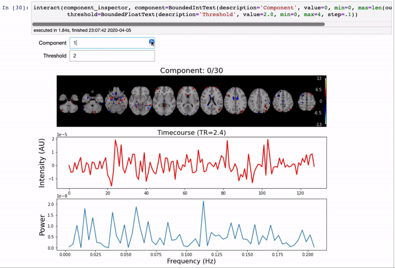
We will use the interactive component_viewer from nltools to explore the results of the analysis. This viewer uses ipywidgets to select the Component to view and also the threshold. You can manually enter a component number to view or scroll up and down.

Components have been standardized, this allows us to threshold the brain in terms of standard deviations. For example, the default threshold of 2.0, means that any voxel that loads on the component greater or less than 2 standard deviations will be overlaid on the standard brain. You can play with different thresholds to be more or less inclusive - a threshold of 0 will overlay all of the voxels. If you play with any of the numbers, make sure you press tab to update the plot.

The second plot is the time course of the voxels that load on the component. The x-axis is in TRs, which for this dataset is 2.4 sec.

The third plot is the powerspectrum of the timecourse. There is not a large range of possible values as we can only observe signals at the nyquist frequency, which is half of our sampling frequency of 1/2.4s (approximately 0.21hz) to a lower bound of 0.0078hz based on our high pass filter. There might be systematic oscillatory signals. Remember, that signals that oscillate a faster frequency than the nyquist frequency will be aliased. This includes physiological artifacts such as respiration and cardiac signals.

It is important to note that ICA cannot resolve the sign of the component. So make sure you consider signals that are positive as well as negative.

component_viewer(output, tr=2.4)

Exercises#

For this tutorial, try to guess which components are signal and which are noise. Also, be sure to label the type of noise you think you might be seeing (e.g., head motion, scanner spikes, cardiac, respiration, etc.) Do this for subjects s01 and s02.

What features do you think are important to consider when making this judgment? Does the spatial map provide any useful information? What about the timecourse of the component? Does it map on to the plausible timecourse of the task.What about the power spectrum?