Introduction to Pandas#
Written by Luke Chang & Jin Cheong
Analyzing data requires being facile with manipulating and transforming datasets to be able to test specific hypotheses. Data come in all different types of flavors and there are many different tools in the Python ecosystem to work with pretty much any type of data you might encounter. For example, you might be interested in working with functional neuroimaging data that is four dimensional. Three dimensional matrices contain brain activations in space, and these data can change over time in the 4th dimension. This type of data is well suited for numpy and specialized brain imaging packages such as nilearn. The majority of data, however, is typically in some version of a two-dimensional observations by features format as might be seen in an excel spreadsheet, a SQL table, or in a comma delimited format (i.e., csv).
In Python, the Pandas library is a powerful tool to work with this type of data. This is a very large library with a tremendous amount of functionality. In this tutorial, we will cover the basics of how to load and manipulate data and will focus on common to data munging tasks.
For those interested in diving deeper into Pandas, there are many online resources. There is the Pandas online documention, stackoverflow, and medium blogposts. I highly recommend Jake Vanderplas’s terrific Python Data Science Handbook. In addition, here is a brief video by Tal Yarkoni providing a useful introduction to pandas.
After the tutorial you will have the chance to apply the methods to a new set of data.
Pandas Objects#
Pandas has several objects that are commonly used (i.e., Series, DataFrame, Index). At it’s core, Pandas Objects are enhanced numpy arrays where columns and rows can have special names and there are lots of methods to operate on the data. See Jake Vanderplas’s tutorial for a more in depth overview.
Series#
A pandas Series is a one-dimensional array of indexed data.
import pandas as pd

data = pd.Series([1, 2, 3, 4, 5])
data
0    1
1    2
2    3
3    4
4    5
dtype: int64
The indices can be integers like in the example above. Alternatively, the indices can be labels.
data = pd.Series([1,2,3], index=['a', 'b', 'c'])
data
a    1
b    2
c    3
dtype: int64
Also, Series can be easily created from dictionaries
data = pd.Series({'A':5, 'B':3, 'C':1})
data
A    5
B    3
C    1
dtype: int64
DataFrame#
If a Series is a one-dimensional indexed array, the DataFrame is a two-dimensional indexed array. It can be thought of as a collection of Series objects, where each Series represents a column, or as an enhanced 2D numpy array.
In a DataFrame, the index refers to labels for each row, while columns describe each column.
First, let’s create a DataFrame using random numbers generated from numpy.
import numpy as np

data = pd.DataFrame(np.random.random((5, 3)))
data
| 0 | 1 | 2 | |
|---|---|---|---|
| 0 | 0.828627 | 0.860628 | 0.239354 |
| 1 | 0.701561 | 0.990040 | 0.955123 |
| 2 | 0.526356 | 0.573977 | 0.854763 |
| 3 | 0.360077 | 0.396195 | 0.303766 |
| 4 | 0.188879 | 0.446423 | 0.063622 |
We could also initialize with column names
data = pd.DataFrame(np.random.random((5, 3)), columns=['A', 'B', 'C'])
data
| A | B | C | |
|---|---|---|---|
| 0 | 0.493188 | 0.513151 | 0.500130 |
| 1 | 0.706082 | 0.967668 | 0.762955 |
| 2 | 0.853237 | 0.361205 | 0.297108 |
| 3 | 0.021289 | 0.920400 | 0.609904 |
| 4 | 0.917379 | 0.207424 | 0.451640 |
Alternatively, we could create a DataFrame from multiple Series objects.
a = pd.Series([1, 2, 3, 4])
b = pd.Series(['a', 'b', 'c', 'd'])
data = pd.DataFrame({'Numbers':a, 'Letters':b})
data
| Numbers | Letters | |
|---|---|---|
| 0 | 1 | a |
| 1 | 2 | b |
| 2 | 3 | c |
| 3 | 4 | d |
Or a python dictionary
data = pd.DataFrame({'State':['California', 'Colorado', 'New Hampshire'],
                     'Capital':['Sacremento', 'Denver', 'Concord']})
data
| State | Capital | |
|---|---|---|
| 0 | California | Sacremento |
| 1 | Colorado | Denver |
| 2 | New Hampshire | Concord |
Loading Data#
Loading data is fairly straightfoward in Pandas. Type pd.read then press tab to see a list of functions that can load specific file formats such as: csv, excel, spss, and sql.
In this example, we will use pd.read_csv to load a .csv file into a dataframe.
Note that read_csv() has many options that can be used to make sure you load the data correctly. You can explore the docstrings for a function to get more information about the inputs and general useage guidelines by running pd.read_csv?
pd.read_csv?
Signature:
pd.read_csv(
    filepath_or_buffer: 'FilePath | ReadCsvBuffer[bytes] | ReadCsvBuffer[str]',
    *,
    sep: 'str | None | lib.NoDefault' = <no_default>,
    delimiter: 'str | None | lib.NoDefault' = None,
    header: "int | Sequence[int] | None | Literal['infer']" = 'infer',
    names: 'Sequence[Hashable] | None | lib.NoDefault' = <no_default>,
    index_col: 'IndexLabel | Literal[False] | None' = None,
    usecols: 'UsecolsArgType' = None,
    dtype: 'DtypeArg | None' = None,
    engine: 'CSVEngine | None' = None,
    converters: 'Mapping[Hashable, Callable] | None' = None,
    true_values: 'list | None' = None,
    false_values: 'list | None' = None,
    skipinitialspace: 'bool' = False,
    skiprows: 'list[int] | int | Callable[[Hashable], bool] | None' = None,
    skipfooter: 'int' = 0,
    nrows: 'int | None' = None,
    na_values: 'Hashable | Iterable[Hashable] | Mapping[Hashable, Iterable[Hashable]] | None' = None,
    keep_default_na: 'bool' = True,
    na_filter: 'bool' = True,
    verbose: 'bool | lib.NoDefault' = <no_default>,
    skip_blank_lines: 'bool' = True,
    parse_dates: 'bool | Sequence[Hashable] | None' = None,
    infer_datetime_format: 'bool | lib.NoDefault' = <no_default>,
    keep_date_col: 'bool | lib.NoDefault' = <no_default>,
    date_parser: 'Callable | lib.NoDefault' = <no_default>,
    date_format: 'str | dict[Hashable, str] | None' = None,
    dayfirst: 'bool' = False,
    cache_dates: 'bool' = True,
    iterator: 'bool' = False,
    chunksize: 'int | None' = None,
    compression: 'CompressionOptions' = 'infer',
    thousands: 'str | None' = None,
    decimal: 'str' = '.',
    lineterminator: 'str | None' = None,
    quotechar: 'str' = '"',
    quoting: 'int' = 0,
    doublequote: 'bool' = True,
    escapechar: 'str | None' = None,
    comment: 'str | None' = None,
    encoding: 'str | None' = None,
    encoding_errors: 'str | None' = 'strict',
    dialect: 'str | csv.Dialect | None' = None,
    on_bad_lines: 'str' = 'error',
    delim_whitespace: 'bool | lib.NoDefault' = <no_default>,
    low_memory: 'bool' = True,
    memory_map: 'bool' = False,
    float_precision: "Literal['high', 'legacy'] | None" = None,
    storage_options: 'StorageOptions | None' = None,
    dtype_backend: 'DtypeBackend | lib.NoDefault' = <no_default>,
) -> 'DataFrame | TextFileReader'
Docstring:
Read a comma-separated values (csv) file into DataFrame.

Also supports optionally iterating or breaking of the file
into chunks.

Additional help can be found in the online docs for
`IO Tools <https://pandas.pydata.org/pandas-docs/stable/user_guide/io.html>`_.

Parameters
----------
filepath_or_buffer : str, path object or file-like object
    Any valid string path is acceptable. The string could be a URL. Valid
    URL schemes include http, ftp, s3, gs, and file. For file URLs, a host is
    expected. A local file could be: file://localhost/path/to/table.csv.

    If you want to pass in a path object, pandas accepts any ``os.PathLike``.

    By file-like object, we refer to objects with a ``read()`` method, such as
    a file handle (e.g. via builtin ``open`` function) or ``StringIO``.
sep : str, default ','
    Character or regex pattern to treat as the delimiter. If ``sep=None``, the
    C engine cannot automatically detect
    the separator, but the Python parsing engine can, meaning the latter will
    be used and automatically detect the separator from only the first valid
    row of the file by Python's builtin sniffer tool, ``csv.Sniffer``.
    In addition, separators longer than 1 character and different from
    ``'\s+'`` will be interpreted as regular expressions and will also force
    the use of the Python parsing engine. Note that regex delimiters are prone
    to ignoring quoted data. Regex example: ``'\r\t'``.
delimiter : str, optional
    Alias for ``sep``.
header : int, Sequence of int, 'infer' or None, default 'infer'
    Row number(s) containing column labels and marking the start of the
    data (zero-indexed). Default behavior is to infer the column names: if no ``names``
    are passed the behavior is identical to ``header=0`` and column
    names are inferred from the first line of the file, if column
    names are passed explicitly to ``names`` then the behavior is identical to
    ``header=None``. Explicitly pass ``header=0`` to be able to
    replace existing names. The header can be a list of integers that
    specify row locations for a :class:`~pandas.MultiIndex` on the columns
    e.g. ``[0, 1, 3]``. Intervening rows that are not specified will be
    skipped (e.g. 2 in this example is skipped). Note that this
    parameter ignores commented lines and empty lines if
    ``skip_blank_lines=True``, so ``header=0`` denotes the first line of
    data rather than the first line of the file.
names : Sequence of Hashable, optional
    Sequence of column labels to apply. If the file contains a header row,
    then you should explicitly pass ``header=0`` to override the column names.
    Duplicates in this list are not allowed.
index_col : Hashable, Sequence of Hashable or False, optional
  Column(s) to use as row label(s), denoted either by column labels or column
  indices.  If a sequence of labels or indices is given, :class:`~pandas.MultiIndex`
  will be formed for the row labels.

  Note: ``index_col=False`` can be used to force pandas to *not* use the first
  column as the index, e.g., when you have a malformed file with delimiters at
  the end of each line.
usecols : Sequence of Hashable or Callable, optional
    Subset of columns to select, denoted either by column labels or column indices.
    If list-like, all elements must either
    be positional (i.e. integer indices into the document columns) or strings
    that correspond to column names provided either by the user in ``names`` or
    inferred from the document header row(s). If ``names`` are given, the document
    header row(s) are not taken into account. For example, a valid list-like
    ``usecols`` parameter would be ``[0, 1, 2]`` or ``['foo', 'bar', 'baz']``.
    Element order is ignored, so ``usecols=[0, 1]`` is the same as ``[1, 0]``.
    To instantiate a :class:`~pandas.DataFrame` from ``data`` with element order
    preserved use ``pd.read_csv(data, usecols=['foo', 'bar'])[['foo', 'bar']]``
    for columns in ``['foo', 'bar']`` order or
    ``pd.read_csv(data, usecols=['foo', 'bar'])[['bar', 'foo']]``
    for ``['bar', 'foo']`` order.

    If callable, the callable function will be evaluated against the column
    names, returning names where the callable function evaluates to ``True``. An
    example of a valid callable argument would be ``lambda x: x.upper() in
    ['AAA', 'BBB', 'DDD']``. Using this parameter results in much faster
    parsing time and lower memory usage.
dtype : dtype or dict of {Hashable : dtype}, optional
    Data type(s) to apply to either the whole dataset or individual columns.
    E.g., ``{'a': np.float64, 'b': np.int32, 'c': 'Int64'}``
    Use ``str`` or ``object`` together with suitable ``na_values`` settings
    to preserve and not interpret ``dtype``.
    If ``converters`` are specified, they will be applied INSTEAD
    of ``dtype`` conversion.

    .. versionadded:: 1.5.0

        Support for ``defaultdict`` was added. Specify a ``defaultdict`` as input where
        the default determines the ``dtype`` of the columns which are not explicitly
        listed.
engine : {'c', 'python', 'pyarrow'}, optional
    Parser engine to use. The C and pyarrow engines are faster, while the python engine
    is currently more feature-complete. Multithreading is currently only supported by
    the pyarrow engine.

    .. versionadded:: 1.4.0

        The 'pyarrow' engine was added as an *experimental* engine, and some features
        are unsupported, or may not work correctly, with this engine.
converters : dict of {Hashable : Callable}, optional
    Functions for converting values in specified columns. Keys can either
    be column labels or column indices.
true_values : list, optional
    Values to consider as ``True`` in addition to case-insensitive variants of 'True'.
false_values : list, optional
    Values to consider as ``False`` in addition to case-insensitive variants of 'False'.
skipinitialspace : bool, default False
    Skip spaces after delimiter.
skiprows : int, list of int or Callable, optional
    Line numbers to skip (0-indexed) or number of lines to skip (``int``)
    at the start of the file.

    If callable, the callable function will be evaluated against the row
    indices, returning ``True`` if the row should be skipped and ``False`` otherwise.
    An example of a valid callable argument would be ``lambda x: x in [0, 2]``.
skipfooter : int, default 0
    Number of lines at bottom of file to skip (Unsupported with ``engine='c'``).
nrows : int, optional
    Number of rows of file to read. Useful for reading pieces of large files.
na_values : Hashable, Iterable of Hashable or dict of {Hashable : Iterable}, optional
    Additional strings to recognize as ``NA``/``NaN``. If ``dict`` passed, specific
    per-column ``NA`` values.  By default the following values are interpreted as
    ``NaN``: " ", "#N/A", "#N/A N/A", "#NA", "-1.#IND", "-1.#QNAN", "-NaN", "-nan",
    "1.#IND", "1.#QNAN", "<NA>", "N/A", "NA", "NULL", "NaN", "None",
    "n/a", "nan", "null ".

keep_default_na : bool, default True
    Whether or not to include the default ``NaN`` values when parsing the data.
    Depending on whether ``na_values`` is passed in, the behavior is as follows:

    * If ``keep_default_na`` is ``True``, and ``na_values`` are specified, ``na_values``
      is appended to the default ``NaN`` values used for parsing.
    * If ``keep_default_na`` is ``True``, and ``na_values`` are not specified, only
      the default ``NaN`` values are used for parsing.
    * If ``keep_default_na`` is ``False``, and ``na_values`` are specified, only
      the ``NaN`` values specified ``na_values`` are used for parsing.
    * If ``keep_default_na`` is ``False``, and ``na_values`` are not specified, no
      strings will be parsed as ``NaN``.

    Note that if ``na_filter`` is passed in as ``False``, the ``keep_default_na`` and
    ``na_values`` parameters will be ignored.
na_filter : bool, default True
    Detect missing value markers (empty strings and the value of ``na_values``). In
    data without any ``NA`` values, passing ``na_filter=False`` can improve the
    performance of reading a large file.
verbose : bool, default False
    Indicate number of ``NA`` values placed in non-numeric columns.

    .. deprecated:: 2.2.0
skip_blank_lines : bool, default True
    If ``True``, skip over blank lines rather than interpreting as ``NaN`` values.
parse_dates : bool, list of Hashable, list of lists or dict of {Hashable : list}, default False
    The behavior is as follows:

    * ``bool``. If ``True`` -> try parsing the index. Note: Automatically set to
      ``True`` if ``date_format`` or ``date_parser`` arguments have been passed.
    * ``list`` of ``int`` or names. e.g. If ``[1, 2, 3]`` -> try parsing columns 1, 2, 3
      each as a separate date column.
    * ``list`` of ``list``. e.g.  If ``[[1, 3]]`` -> combine columns 1 and 3 and parse
      as a single date column. Values are joined with a space before parsing.
    * ``dict``, e.g. ``{'foo' : [1, 3]}`` -> parse columns 1, 3 as date and call
      result 'foo'. Values are joined with a space before parsing.

    If a column or index cannot be represented as an array of ``datetime``,
    say because of an unparsable value or a mixture of timezones, the column
    or index will be returned unaltered as an ``object`` data type. For
    non-standard ``datetime`` parsing, use :func:`~pandas.to_datetime` after
    :func:`~pandas.read_csv`.

    Note: A fast-path exists for iso8601-formatted dates.
infer_datetime_format : bool, default False
    If ``True`` and ``parse_dates`` is enabled, pandas will attempt to infer the
    format of the ``datetime`` strings in the columns, and if it can be inferred,
    switch to a faster method of parsing them. In some cases this can increase
    the parsing speed by 5-10x.

    .. deprecated:: 2.0.0
        A strict version of this argument is now the default, passing it has no effect.

keep_date_col : bool, default False
    If ``True`` and ``parse_dates`` specifies combining multiple columns then
    keep the original columns.
date_parser : Callable, optional
    Function to use for converting a sequence of string columns to an array of
    ``datetime`` instances. The default uses ``dateutil.parser.parser`` to do the
    conversion. pandas will try to call ``date_parser`` in three different ways,
    advancing to the next if an exception occurs: 1) Pass one or more arrays
    (as defined by ``parse_dates``) as arguments; 2) concatenate (row-wise) the
    string values from the columns defined by ``parse_dates`` into a single array
    and pass that; and 3) call ``date_parser`` once for each row using one or
    more strings (corresponding to the columns defined by ``parse_dates``) as
    arguments.

    .. deprecated:: 2.0.0
       Use ``date_format`` instead, or read in as ``object`` and then apply
       :func:`~pandas.to_datetime` as-needed.
date_format : str or dict of column -> format, optional
    Format to use for parsing dates when used in conjunction with ``parse_dates``.
    The strftime to parse time, e.g. :const:`"%d/%m/%Y"`. See
    `strftime documentation
    <https://docs.python.org/3/library/datetime.html
    #strftime-and-strptime-behavior>`_ for more information on choices, though
    note that :const:`"%f"` will parse all the way up to nanoseconds.
    You can also pass:

    - "ISO8601", to parse any `ISO8601 <https://en.wikipedia.org/wiki/ISO_8601>`_
        time string (not necessarily in exactly the same format);
    - "mixed", to infer the format for each element individually. This is risky,
        and you should probably use it along with `dayfirst`.

    .. versionadded:: 2.0.0
dayfirst : bool, default False
    DD/MM format dates, international and European format.
cache_dates : bool, default True
    If ``True``, use a cache of unique, converted dates to apply the ``datetime``
    conversion. May produce significant speed-up when parsing duplicate
    date strings, especially ones with timezone offsets.

iterator : bool, default False
    Return ``TextFileReader`` object for iteration or getting chunks with
    ``get_chunk()``.
chunksize : int, optional
    Number of lines to read from the file per chunk. Passing a value will cause the
    function to return a ``TextFileReader`` object for iteration.
    See the `IO Tools docs
    <https://pandas.pydata.org/pandas-docs/stable/io.html#io-chunking>`_
    for more information on ``iterator`` and ``chunksize``.

compression : str or dict, default 'infer'
    For on-the-fly decompression of on-disk data. If 'infer' and 'filepath_or_buffer' is
    path-like, then detect compression from the following extensions: '.gz',
    '.bz2', '.zip', '.xz', '.zst', '.tar', '.tar.gz', '.tar.xz' or '.tar.bz2'
    (otherwise no compression).
    If using 'zip' or 'tar', the ZIP file must contain only one data file to be read in.
    Set to ``None`` for no decompression.
    Can also be a dict with key ``'method'`` set
    to one of {``'zip'``, ``'gzip'``, ``'bz2'``, ``'zstd'``, ``'xz'``, ``'tar'``} and
    other key-value pairs are forwarded to
    ``zipfile.ZipFile``, ``gzip.GzipFile``,
    ``bz2.BZ2File``, ``zstandard.ZstdDecompressor``, ``lzma.LZMAFile`` or
    ``tarfile.TarFile``, respectively.
    As an example, the following could be passed for Zstandard decompression using a
    custom compression dictionary:
    ``compression={'method': 'zstd', 'dict_data': my_compression_dict}``.

    .. versionadded:: 1.5.0
        Added support for `.tar` files.

    .. versionchanged:: 1.4.0 Zstandard support.

thousands : str (length 1), optional
    Character acting as the thousands separator in numerical values.
decimal : str (length 1), default '.'
    Character to recognize as decimal point (e.g., use ',' for European data).
lineterminator : str (length 1), optional
    Character used to denote a line break. Only valid with C parser.
quotechar : str (length 1), optional
    Character used to denote the start and end of a quoted item. Quoted
    items can include the ``delimiter`` and it will be ignored.
quoting : {0 or csv.QUOTE_MINIMAL, 1 or csv.QUOTE_ALL, 2 or csv.QUOTE_NONNUMERIC, 3 or csv.QUOTE_NONE}, default csv.QUOTE_MINIMAL
    Control field quoting behavior per ``csv.QUOTE_*`` constants. Default is
    ``csv.QUOTE_MINIMAL`` (i.e., 0) which implies that only fields containing special
    characters are quoted (e.g., characters defined in ``quotechar``, ``delimiter``,
    or ``lineterminator``.
doublequote : bool, default True
   When ``quotechar`` is specified and ``quoting`` is not ``QUOTE_NONE``, indicate
   whether or not to interpret two consecutive ``quotechar`` elements INSIDE a
   field as a single ``quotechar`` element.
escapechar : str (length 1), optional
    Character used to escape other characters.
comment : str (length 1), optional
    Character indicating that the remainder of line should not be parsed.
    If found at the beginning
    of a line, the line will be ignored altogether. This parameter must be a
    single character. Like empty lines (as long as ``skip_blank_lines=True``),
    fully commented lines are ignored by the parameter ``header`` but not by
    ``skiprows``. For example, if ``comment='#'``, parsing
    ``#empty\na,b,c\n1,2,3`` with ``header=0`` will result in ``'a,b,c'`` being
    treated as the header.
encoding : str, optional, default 'utf-8'
    Encoding to use for UTF when reading/writing (ex. ``'utf-8'``). `List of Python
    standard encodings
    <https://docs.python.org/3/library/codecs.html#standard-encodings>`_ .

encoding_errors : str, optional, default 'strict'
    How encoding errors are treated. `List of possible values
    <https://docs.python.org/3/library/codecs.html#error-handlers>`_ .

    .. versionadded:: 1.3.0

dialect : str or csv.Dialect, optional
    If provided, this parameter will override values (default or not) for the
    following parameters: ``delimiter``, ``doublequote``, ``escapechar``,
    ``skipinitialspace``, ``quotechar``, and ``quoting``. If it is necessary to
    override values, a ``ParserWarning`` will be issued. See ``csv.Dialect``
    documentation for more details.
on_bad_lines : {'error', 'warn', 'skip'} or Callable, default 'error'
    Specifies what to do upon encountering a bad line (a line with too many fields).
    Allowed values are :

    - ``'error'``, raise an Exception when a bad line is encountered.
    - ``'warn'``, raise a warning when a bad line is encountered and skip that line.
    - ``'skip'``, skip bad lines without raising or warning when they are encountered.

    .. versionadded:: 1.3.0

    .. versionadded:: 1.4.0

        - Callable, function with signature
          ``(bad_line: list[str]) -> list[str] | None`` that will process a single
          bad line. ``bad_line`` is a list of strings split by the ``sep``.
          If the function returns ``None``, the bad line will be ignored.
          If the function returns a new ``list`` of strings with more elements than
          expected, a ``ParserWarning`` will be emitted while dropping extra elements.
          Only supported when ``engine='python'``

    .. versionchanged:: 2.2.0

        - Callable, function with signature
          as described in `pyarrow documentation
          <https://arrow.apache.org/docs/python/generated/pyarrow.csv.ParseOptions.html
          #pyarrow.csv.ParseOptions.invalid_row_handler>`_ when ``engine='pyarrow'``

delim_whitespace : bool, default False
    Specifies whether or not whitespace (e.g. ``' '`` or ``'\t'``) will be
    used as the ``sep`` delimiter. Equivalent to setting ``sep='\s+'``. If this option
    is set to ``True``, nothing should be passed in for the ``delimiter``
    parameter.

    .. deprecated:: 2.2.0
        Use ``sep="\s+"`` instead.
low_memory : bool, default True
    Internally process the file in chunks, resulting in lower memory use
    while parsing, but possibly mixed type inference.  To ensure no mixed
    types either set ``False``, or specify the type with the ``dtype`` parameter.
    Note that the entire file is read into a single :class:`~pandas.DataFrame`
    regardless, use the ``chunksize`` or ``iterator`` parameter to return the data in
    chunks. (Only valid with C parser).
memory_map : bool, default False
    If a filepath is provided for ``filepath_or_buffer``, map the file object
    directly onto memory and access the data directly from there. Using this
    option can improve performance because there is no longer any I/O overhead.
float_precision : {'high', 'legacy', 'round_trip'}, optional
    Specifies which converter the C engine should use for floating-point
    values. The options are ``None`` or ``'high'`` for the ordinary converter,
    ``'legacy'`` for the original lower precision pandas converter, and
    ``'round_trip'`` for the round-trip converter.

storage_options : dict, optional
    Extra options that make sense for a particular storage connection, e.g.
    host, port, username, password, etc. For HTTP(S) URLs the key-value pairs
    are forwarded to ``urllib.request.Request`` as header options. For other
    URLs (e.g. starting with "s3://", and "gcs://") the key-value pairs are
    forwarded to ``fsspec.open``. Please see ``fsspec`` and ``urllib`` for more
    details, and for more examples on storage options refer `here
    <https://pandas.pydata.org/docs/user_guide/io.html?
    highlight=storage_options#reading-writing-remote-files>`_.

dtype_backend : {'numpy_nullable', 'pyarrow'}, default 'numpy_nullable'
    Back-end data type applied to the resultant :class:`DataFrame`
    (still experimental). Behaviour is as follows:

    * ``"numpy_nullable"``: returns nullable-dtype-backed :class:`DataFrame`
      (default).
    * ``"pyarrow"``: returns pyarrow-backed nullable :class:`ArrowDtype`
      DataFrame.

    .. versionadded:: 2.0

Returns
-------
DataFrame or TextFileReader
    A comma-separated values (csv) file is returned as two-dimensional
    data structure with labeled axes.

See Also
--------
DataFrame.to_csv : Write DataFrame to a comma-separated values (csv) file.
read_table : Read general delimited file into DataFrame.
read_fwf : Read a table of fixed-width formatted lines into DataFrame.

Examples
--------
>>> pd.read_csv('data.csv')  # doctest: +SKIP
File:      /opt/anaconda3/envs/py312/lib/python3.12/site-packages/pandas/io/parsers/readers.py
Type:      function
To load a csv file we will need to specify either the relative or absolute path to the file.
The command pwd will print the path of the current working directory.
pwd
'/Users/lukechang/Github/dartbrains/content'
We will now load the Pandas has many ways to read data different data formats into a dataframe. Here we will use the pd.read_csv function.
df = pd.read_csv('https://raw.githubusercontent.com/ljchang/dartbrains/master/data/salary/salary.csv', sep = ',')
Ways to check the dataframe#
There are many ways to examine your dataframe. One easy way is to just call the dataframe variable itself.
df
| salary | gender | departm | years | age | publications | |
|---|---|---|---|---|---|---|
| 0 | 86285 | 0 | bio | 26.0 | 64.0 | 72 |
| 1 | 77125 | 0 | bio | 28.0 | 58.0 | 43 |
| 2 | 71922 | 0 | bio | 10.0 | 38.0 | 23 |
| 3 | 70499 | 0 | bio | 16.0 | 46.0 | 64 |
| 4 | 66624 | 0 | bio | 11.0 | 41.0 | 23 |
| ... | ... | ... | ... | ... | ... | ... |
| 72 | 53662 | 1 | neuro | 1.0 | 31.0 | 3 |
| 73 | 57185 | 1 | stat | 9.0 | 39.0 | 7 |
| 74 | 52254 | 1 | stat | 2.0 | 32.0 | 9 |
| 75 | 61885 | 1 | math | 23.0 | 60.0 | 9 |
| 76 | 49542 | 1 | math | 3.0 | 33.0 | 5 |
77 rows × 6 columns
However, often the dataframes can be large and we may be only interested in seeing the first few rows. df.head() is useful for this purpose.
df.head()
| salary | gender | departm | years | age | publications | |
|---|---|---|---|---|---|---|
| 0 | 86285 | 0 | bio | 26.0 | 64.0 | 72 |
| 1 | 77125 | 0 | bio | 28.0 | 58.0 | 43 |
| 2 | 71922 | 0 | bio | 10.0 | 38.0 | 23 |
| 3 | 70499 | 0 | bio | 16.0 | 46.0 | 64 |
| 4 | 66624 | 0 | bio | 11.0 | 41.0 | 23 |
On the top row, you have column names, that can be called like a dictionary (a dataframe can be essentially thought of as a dictionary with column names as the keys). The left most column (0,1,2,3,4…) is called the index of the dataframe. The default index is sequential integers, but it can be set to anything as long as each row is unique (e.g., subject IDs)
print("Indexes")
print(df.index)
print("Columns")
print(df.columns)
print("Columns are like keys of a dictionary")
print(df.keys())
Indexes
RangeIndex(start=0, stop=77, step=1)
Columns
Index(['salary', 'gender', 'departm', 'years', 'age', 'publications'], dtype='object')
Columns are like keys of a dictionary
Index(['salary', 'gender', 'departm', 'years', 'age', 'publications'], dtype='object')
You can access the values of a column by calling it directly. Single bracket returns a Series and double bracket returns a dataframe.
Let’s return the first 10 rows of salary.
df['salary'][:10]
0    86285
1    77125
2    71922
3    70499
4    66624
5    64451
6    64366
7    59344
8    58560
9    58294
Name: salary, dtype: int64
shape is another useful method for getting the dimensions of the matrix.
We will print the number of rows and columns in this data set using fstring formatting. First, you need to specify a string starting with ‘f’, like this f'anything'. It is easy to insert variables with curly brackets like this f'rows: {rows}'.
Here is more info about formatting text.
rows, cols = df.shape
print(f'There are {rows} rows and {cols} columns in this data set')
There are 77 rows and 6 columns in this data set
Describing the data#
We can use the .describe() method to get a quick summary of the continuous values of the data frame. We will .transpose() the output to make it slightly easier to read.
df.describe().transpose()
| count | mean | std | min | 25% | 50% | 75% | max | |
|---|---|---|---|---|---|---|---|---|
| salary | 77.0 | 67748.519481 | 15100.581435 | 44687.0 | 57185.0 | 62607.0 | 75382.0 | 112800.0 |
| gender | 77.0 | 0.142857 | 0.387783 | 0.0 | 0.0 | 0.0 | 0.0 | 2.0 |
| years | 76.0 | 14.973684 | 8.617770 | 1.0 | 8.0 | 14.0 | 23.0 | 34.0 |
| age | 76.0 | 45.486842 | 9.005914 | 31.0 | 38.0 | 44.0 | 53.0 | 65.0 |
| publications | 77.0 | 21.831169 | 15.240530 | 3.0 | 9.0 | 19.0 | 33.0 | 72.0 |
We can also get quick summary of a pandas series, or specific column of a pandas dataframe.
df.departm.describe()
count      77
unique      7
top       bio
freq       16
Name: departm, dtype: object
Sometimes, you will want to know how many data points are associated with a specific variable for categorical data. The value_counts method can be used for this goal.
For example, how many males and females are in this dataset?
df['gender'].value_counts()
gender
0    67
1     9
2     1
Name: count, dtype: int64
You can see that there are more than 2 genders specified in our data.
This is likely an error in the data collection process. It’s always up to the data analyst to decide what to do in these cases. Because we don’t know what the true value should have been, let’s just remove the row from the dataframe by finding all rows that are not ‘2’.
df = df.loc[df['gender']!=2]

df['gender'].value_counts()
gender
0    67
1     9
Name: count, dtype: int64
Dealing with missing values#
Data are always messy and often have lots of missing values. There are many different ways, in which missing data might present NaN, None, or NA, Sometimes researchers code missing values with specific numeric codes such as 999999. It is important to find these as they can screw up your analyses if they are hiding in your data.
If the missing values are using a standard pandas or numpy value such as NaN, None, or NA, we can identify where the missing values are as booleans using the isnull() method.
The isnull() method will return a dataframe with True/False values on whether a datapoint is null or not a number (nan).
df.isnull()
| salary | gender | departm | years | age | publications | |
|---|---|---|---|---|---|---|
| 0 | False | False | False | False | False | False |
| 1 | False | False | False | False | False | False |
| 2 | False | False | False | False | False | False |
| 3 | False | False | False | False | False | False |
| 4 | False | False | False | False | False | False |
| ... | ... | ... | ... | ... | ... | ... |
| 72 | False | False | False | False | False | False |
| 73 | False | False | False | False | False | False |
| 74 | False | False | False | False | False | False |
| 75 | False | False | False | False | False | False |
| 76 | False | False | False | False | False | False |
76 rows × 6 columns
Suppose we wanted to count the number of missing values for each column in the dataset.
One thing that is nice about Python is that you can chain commands, which means that the output of one method can be the input into the next method. This allows us to write intuitive and concise code. Notice how we take the sum() of all of the null cases.
We can chain the .null() and .sum() methods to see how many null values are added up in each column.
df.isnull().sum()
salary          0
gender          0
departm         0
years           1
age             1
publications    0
dtype: int64
You can use the boolean indexing once again to see the datapoints that have missing values. We chained the method .any() which will check if there are any True values for a given axis. Axis=0 indicates rows, while Axis=1 indicates columns. So here we are creating a boolean index for row where any column has a missing value.
df[df.isnull().any(axis=1)]
| salary | gender | departm | years | age | publications | |
|---|---|---|---|---|---|---|
| 18 | 64762 | 0 | chem | 25.0 | NaN | 29 |
| 24 | 104828 | 0 | geol | NaN | 50.0 | 44 |
You may look at where the values are not null. Note that indexes 18, and 24 are missing.
df[~df.isnull().any(axis=1)]
| salary | gender | departm | years | age | publications | |
|---|---|---|---|---|---|---|
| 0 | 86285 | 0 | bio | 26.0 | 64.0 | 72 |
| 1 | 77125 | 0 | bio | 28.0 | 58.0 | 43 |
| 2 | 71922 | 0 | bio | 10.0 | 38.0 | 23 |
| 3 | 70499 | 0 | bio | 16.0 | 46.0 | 64 |
| 4 | 66624 | 0 | bio | 11.0 | 41.0 | 23 |
| ... | ... | ... | ... | ... | ... | ... |
| 72 | 53662 | 1 | neuro | 1.0 | 31.0 | 3 |
| 73 | 57185 | 1 | stat | 9.0 | 39.0 | 7 |
| 74 | 52254 | 1 | stat | 2.0 | 32.0 | 9 |
| 75 | 61885 | 1 | math | 23.0 | 60.0 | 9 |
| 76 | 49542 | 1 | math | 3.0 | 33.0 | 5 |
74 rows × 6 columns
There are different techniques for dealing with missing data. An easy one is to simply remove rows that have any missing values using the dropna() method.
df.dropna(inplace=True)
/var/folders/5b/m183lc3x27n9krrzz85z2x1c0000gn/T/ipykernel_28379/1379821321.py:1: SettingWithCopyWarning:
A value is trying to be set on a copy of a slice from a DataFrame

See the caveats in the documentation: https://pandas.pydata.org/pandas-docs/stable/user_guide/indexing.html#returning-a-view-versus-a-copy
  df.dropna(inplace=True)
Now we can check to make sure the missing rows are removed. Let’s also check the new dimensions of the dataframe.
rows, cols = df.shape
print(f'There are {rows} rows and {cols} columns in this data set')

df.isnull().sum()
There are 74 rows and 6 columns in this data set
salary          0
gender          0
departm         0
years           0
age             0
publications    0
dtype: int64
Create New Columns#
You can create new columns to fit your needs. For instance you can set initialize a new column with zeros.
df['pubperyear'] = 0
/var/folders/5b/m183lc3x27n9krrzz85z2x1c0000gn/T/ipykernel_28379/2945664157.py:1: SettingWithCopyWarning:
A value is trying to be set on a copy of a slice from a DataFrame.
Try using .loc[row_indexer,col_indexer] = value instead

See the caveats in the documentation: https://pandas.pydata.org/pandas-docs/stable/user_guide/indexing.html#returning-a-view-versus-a-copy
  df['pubperyear'] = 0
Here we can create a new column pubperyear, which is the ratio of the number of papers published per year
df['pubperyear'] = df['publications']/df['years']
/var/folders/5b/m183lc3x27n9krrzz85z2x1c0000gn/T/ipykernel_28379/1818352125.py:1: SettingWithCopyWarning:
A value is trying to be set on a copy of a slice from a DataFrame.
Try using .loc[row_indexer,col_indexer] = value instead

See the caveats in the documentation: https://pandas.pydata.org/pandas-docs/stable/user_guide/indexing.html#returning-a-view-versus-a-copy
  df['pubperyear'] = df['publications']/df['years']
Indexing and slicing Data#
Indexing in Pandas can be tricky. There are many ways to index in pandas, for this tutorial we will focus on four: loc, iloc, boolean, and indexing numpy values. For a more in depth overview see Jake Vanderplas’s tutorial](jakevdp/PythonDataScienceHandbook), where he also covers more advanced topics, such as hierarchical indexing.
Indexing with Keys#
First, we will cover indexing with keys using the .loc method. This method references the explicit index with a key name. It works for both index names and also column names. Note that often the keys for rows are integers by default.
In this example, we will return rows 10-20 on the salary column.
df.loc[10:20, 'salary']
10    56092
11    54452
12    54269
13    55125
14    97630
15    82444
16    76291
17    75382
19    62607
20    60373
Name: salary, dtype: int64
You can return multiple columns using a list.
df.loc[:10, ['salary', 'publications']]
| salary | publications | |
|---|---|---|
| 0 | 86285 | 72 |
| 1 | 77125 | 43 |
| 2 | 71922 | 23 |
| 3 | 70499 | 64 |
| 4 | 66624 | 23 |
| 5 | 64451 | 44 |
| 6 | 64366 | 22 |
| 7 | 59344 | 11 |
| 8 | 58560 | 8 |
| 9 | 58294 | 12 |
| 10 | 56092 | 4 |
Indexing with Integers#
Next we wil try .iloc. This method references the implicit python index using integer indexing (starting from 0, exclusive of last number). You can think of this like row by column indexing using integers.
For example, let’s grab the first 3 rows and columns.
df.iloc[0:3, 0:3]
| salary | gender | departm | |
|---|---|---|---|
| 0 | 86285 | 0 | bio |
| 1 | 77125 | 0 | bio |
| 2 | 71922 | 0 | bio |
Let’s make a new data frame with just Males and another for just Females. Notice, how we added the .reset_index(drop=True) method? This is because assigning a new dataframe based on indexing another dataframe will retain the original index. We need to explicitly tell pandas to reset the index if we want it to start from zero.
male_df = df[df.gender == 0].reset_index(drop=True)
female_df = df[df.gender == 1].reset_index(drop=True)
Indexing with booleans#
Boolean or logical indexing is useful if you need to sort the data based on some True or False value.
For instance, who are the people with salaries greater than 90K but lower than 100K ?
df[ (df.salary > 90000) & (df.salary < 100000)]
| salary | gender | departm | years | age | publications | pubperyear | |
|---|---|---|---|---|---|---|---|
| 14 | 97630 | 0 | chem | 34.0 | 64.0 | 43 | 1.264706 |
| 30 | 92951 | 0 | neuro | 11.0 | 41.0 | 20 | 1.818182 |
| 54 | 96936 | 0 | physics | 15.0 | 50.0 | 17 | 1.133333 |
This also works with the .loc method, which is what you need to do if you want to return specific columns
df.loc[ (df.salary > 90000) & (df.salary < 100000), ['salary', 'gender']]
| salary | gender | |
|---|---|---|
| 14 | 97630 | 0 |
| 30 | 92951 | 0 |
| 54 | 96936 | 0 |
Numpy indexing#
Finally, you can also return a numpy matrix from a pandas data frame by accessing the .values property. This returns a numpy array that can be indexed using numpy integer indexing and slicing.
As an example, let’s grab the last 10 rows and the first 3 columns.
df.values[-10:, :3]
array([[53638, 0, 'math'],
       [59139, 1, 'bio'],
       [52968, 1, 'bio'],
       [55949, 1, 'chem'],
       [58893, 1, 'neuro'],
       [53662, 1, 'neuro'],
       [57185, 1, 'stat'],
       [52254, 1, 'stat'],
       [61885, 1, 'math'],
       [49542, 1, 'math']], dtype=object)
Renaming#
Part of cleaning up the data is renaming with more sensible names. This is easy to do with Pandas.
Renaming Columns#
We can rename columns with the .rename method by passing in a dictionary using the {'Old Name':'New Name'}. We either need to assigne the result to a new variable or add inplace=True.
df.rename({'departm':'department','pubperyear':'pub_per_year'}, axis=1, inplace=True)
/var/folders/5b/m183lc3x27n9krrzz85z2x1c0000gn/T/ipykernel_28379/144029972.py:1: SettingWithCopyWarning:
A value is trying to be set on a copy of a slice from a DataFrame

See the caveats in the documentation: https://pandas.pydata.org/pandas-docs/stable/user_guide/indexing.html#returning-a-view-versus-a-copy
  df.rename({'departm':'department','pubperyear':'pub_per_year'}, axis=1, inplace=True)
Renaming Rows#
Often we may want to change the coding scheme for a variable. For example, it is hard to remember what zeros and ones mean in the gender variable. We can make this easier by changing these with a dictionary {0:'male', 1:'female'} with the replace method. We can do this inplace=True or we can assign it to a new variable. As an example, we will assign this to a new variable to also retain the original lablels.
df['gender_name'] = df['gender'].replace({0:'male', 1:'female'})

df.head()
/var/folders/5b/m183lc3x27n9krrzz85z2x1c0000gn/T/ipykernel_28379/1691057888.py:1: SettingWithCopyWarning:
A value is trying to be set on a copy of a slice from a DataFrame.
Try using .loc[row_indexer,col_indexer] = value instead

See the caveats in the documentation: https://pandas.pydata.org/pandas-docs/stable/user_guide/indexing.html#returning-a-view-versus-a-copy
  df['gender_name'] = df['gender'].replace({0:'male', 1:'female'})
| salary | gender | department | years | age | publications | pub_per_year | gender_name | |
|---|---|---|---|---|---|---|---|---|
| 0 | 86285 | 0 | bio | 26.0 | 64.0 | 72 | 2.769231 | male |
| 1 | 77125 | 0 | bio | 28.0 | 58.0 | 43 | 1.535714 | male |
| 2 | 71922 | 0 | bio | 10.0 | 38.0 | 23 | 2.300000 | male |
| 3 | 70499 | 0 | bio | 16.0 | 46.0 | 64 | 4.000000 | male |
| 4 | 66624 | 0 | bio | 11.0 | 41.0 | 23 | 2.090909 | male |
Operations#
One of the really fun things about pandas once you get the hang of it is how easy it is to perform operations on the data. It is trivial to compute simple summaries of the data. We can also leverage the object-oriented nature of a pandas object, we can chain together multiple commands.
For example, let’s grab the mean of a few columns.
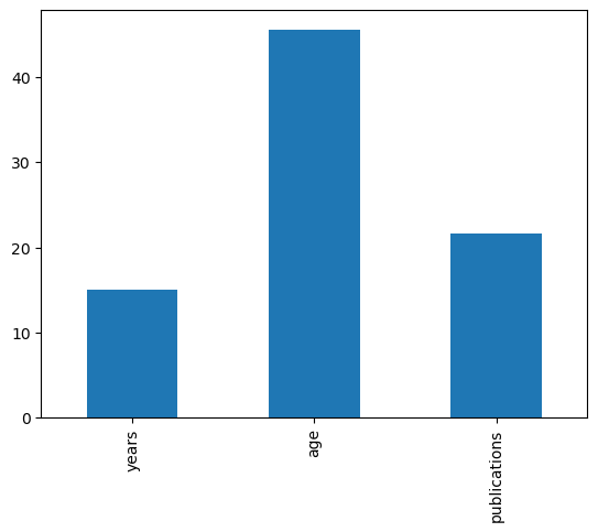
df.loc[:,['years', 'age', 'publications']].mean()
years           14.972973
age             45.567568
publications    21.662162
dtype: float64
We can also turn these values into a plot with the plot method, which we will cover in more detail in future tutorials.
%matplotlib inline

df.loc[:,['years', 'age', 'publications']].mean().plot(kind='bar')
<Axes: >
Perhaps we want to see if there are any correlations in our dataset. We can do this with the .corr method. More recent versions of Pandas might produce an error if there are any columns containing string data. To avoid this issue set numeric_only=True.
df.corr(numeric_only=True)
| salary | gender | years | age | publications | pub_per_year | |
|---|---|---|---|---|---|---|
| salary | 1.000000 | -0.300071 | 0.303275 | 0.275534 | 0.427426 | -0.016988 |
| gender | -0.300071 | 1.000000 | -0.275468 | -0.277098 | -0.249410 | 0.024210 |
| years | 0.303275 | -0.275468 | 1.000000 | 0.958181 | 0.323965 | -0.541125 |
| age | 0.275534 | -0.277098 | 0.958181 | 1.000000 | 0.328285 | -0.498825 |
| publications | 0.427426 | -0.249410 | 0.323965 | 0.328285 | 1.000000 | 0.399865 |
| pub_per_year | -0.016988 | 0.024210 | -0.541125 | -0.498825 | 0.399865 | 1.000000 |
Merging Data#
Another common data manipulation goal is to merge datasets. There are multiple ways to do this in pandas, we will cover concatenation, append, and merge.
Concatenation#
Concatenation describes the process of stacking dataframes together. Older versions of pandas also had an .append() method, which has been deprecated since pandas 1.4. The main thing to consider is to make sure that the shapes of the two dataframes are the same as well as the index labels. For example, if we wanted to vertically stack two dataframe, they need to have the same column names.
Remember that we previously created two separate dataframes for males and females? Let’s put them back together using the pd.concat method. Note how the index of this output retains the old index.
combined_data = pd.concat([female_df, male_df], axis = 0)
We can reset the index using the reset_index method.
pd.concat([male_df, female_df], axis = 0).reset_index(drop=True)
| salary | gender | departm | years | age | publications | pubperyear | |
|---|---|---|---|---|---|---|---|
| 0 | 86285 | 0 | bio | 26.0 | 64.0 | 72 | 2.769231 |
| 1 | 77125 | 0 | bio | 28.0 | 58.0 | 43 | 1.535714 |
| 2 | 71922 | 0 | bio | 10.0 | 38.0 | 23 | 2.300000 |
| 3 | 70499 | 0 | bio | 16.0 | 46.0 | 64 | 4.000000 |
| 4 | 66624 | 0 | bio | 11.0 | 41.0 | 23 | 2.090909 |
| ... | ... | ... | ... | ... | ... | ... | ... |
| 69 | 53662 | 1 | neuro | 1.0 | 31.0 | 3 | 3.000000 |
| 70 | 57185 | 1 | stat | 9.0 | 39.0 | 7 | 0.777778 |
| 71 | 52254 | 1 | stat | 2.0 | 32.0 | 9 | 4.500000 |
| 72 | 61885 | 1 | math | 23.0 | 60.0 | 9 | 0.391304 |
| 73 | 49542 | 1 | math | 3.0 | 33.0 | 5 | 1.666667 |
74 rows × 7 columns
We can also concatenate columns in addition to rows. Make sure that the number of rows are the same in each dataframe. For this example, we will just create two new data frames with a subset of the columns and then combine them again.
df1 = df[['salary', 'gender']]
df2 = df[['age', 'publications']]
df3 = pd.concat([df1, df2], axis=1)
df3.head()
| salary | gender | age | publications | |
|---|---|---|---|---|
| 0 | 86285 | 0 | 64.0 | 72 |
| 1 | 77125 | 0 | 58.0 | 43 |
| 2 | 71922 | 0 | 38.0 | 23 |
| 3 | 70499 | 0 | 46.0 | 64 |
| 4 | 66624 | 0 | 41.0 | 23 |
Merge#
The most powerful method of merging data is using the pd.merge method. This allows you to merge datasets of different shapes and sizes on specific variables that match. This is very common when you need to merge multiple sql tables together for example.
In this example, we are creating two separate data frames that have different states and columns and will merge on the State column.
First, we will only retain rows where there is a match across dataframes, using how=inner. This is equivalent to an ‘and’ join in sql.
df1 = pd.DataFrame({'State':['California', 'Colorado', 'New Hampshire'],
                    'Capital':['Sacremento', 'Denver', 'Concord']})
df2 = pd.DataFrame({'State':['California', 'New Hampshire', 'New York'],
                    'Population':['39512223', '1359711', '19453561']})

df3 = pd.merge(left=df1, right=df2, on='State', how='inner')
df3
| State | Capital | Population | |
|---|---|---|---|
| 0 | California | Sacremento | 39512223 |
| 1 | New Hampshire | Concord | 1359711 |
Notice how there are only two rows in the merged dataframe.
We can also be more inclusive and match on State column, but retain all rows. This is equivalent to an ‘or’ join.
df3 = pd.merge(left=df1, right=df2, on='State', how='outer')
df3
| State | Capital | Population | |
|---|---|---|---|
| 0 | California | Sacremento | 39512223 |
| 1 | Colorado | Denver | NaN |
| 2 | New Hampshire | Concord | 1359711 |
| 3 | New York | NaN | 19453561 |
This is a very handy way to merge data when you have lots of files with missing data. See Jake Vanderplas’s tutorial for a more in depth overview.
Grouping#
We’ve seen above that it is very easy to summarize data over columns using the builtin functions such as pd.mean(). Sometimes we are interested in summarizing data over different groups of rows. For example, what is the mean of participants in Condition A compared to Condition B?
This is suprisingly easy to compute in pandas using the groupby operator, where we aggregate data using a specific operation over different labels.
One useful way to conceptualize this is using the Split, Apply, Combine operation (similar to map-reduce).
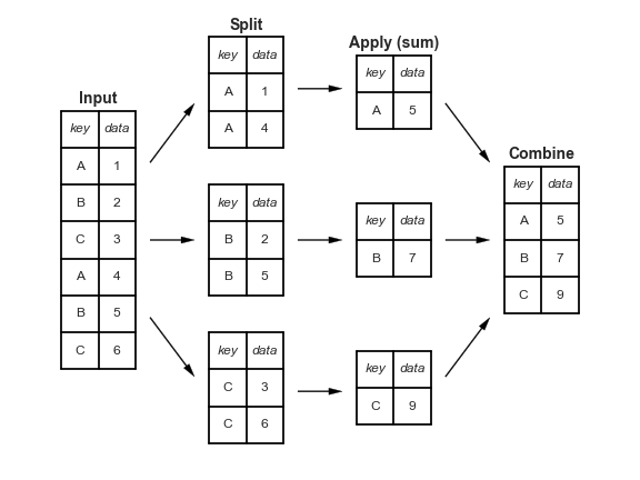
This figure is taken from Jake Vanderplas’s tutorial and highlights how input data can be split on some key and then an operation such as sum can be applied separately to each split. Finally, the results of the applied function for each key can be combined into a new data frame.
Groupby#
In this example, we will use the groupby operator to split the data based on gender labels and separately calculate the mean for each group. Note that newer versions of pandas might throw an error if you try to perform a numeric computation such as .mean() on a dataframe containing columns of string data. Use the flag numeric_only=True to avoid this issue.
df.groupby('gender_name').mean(numeric_only=True)
| salary | gender | years | age | publications | pub_per_year | |
|---|---|---|---|---|---|---|
| gender_name | ||||||
| female | 55719.666667 | 1.0 | 8.666667 | 38.888889 | 11.555556 | 2.043170 |
| male | 69108.492308 | 0.0 | 15.846154 | 46.492308 | 23.061538 | 1.924709 |
Other default aggregation methods include .count(), .mean(), .median(), .min(), .max(), .std(), .var(), and .sum()
Transform#
While the split, apply, combine operation that we just demonstrated is extremely usefuly to quickly summarize data based on a grouping key, the resulting data frame is compressed to one row per grouping label.
Sometimes, we would like to perform an operation over groups, but retain the original data shape. One common example is standardizing data within a subject or grouping variable. Normally, you might think to loop over subject ids and separately z-score or center a variable and then recombine the subject data using a vertical concatenation operation.
The transform method in pandas can make this much easier and faster!
Suppose we want to compute the standardized salary separately for each department. We can standardize using a z-score which requires subtracting the departmental mean from each professor’s salary in that department, and then dividing it by the departmental standard deviation.
We can do this by using the groupby(key) method chained with the .transform(function) method. It will group the dataframe by the key column, perform the “function” transformation of the data and return data in same format. We can then assign the results to a new column in the dataframe.
df['salary_dept_z'] = (df['salary'] - df['salary'].groupby(df['department']).transform('mean'))/df['salary'].groupby(df['department']).transform('std')
df.head()
/var/folders/5b/m183lc3x27n9krrzz85z2x1c0000gn/T/ipykernel_28379/2225281835.py:1: SettingWithCopyWarning:
A value is trying to be set on a copy of a slice from a DataFrame.
Try using .loc[row_indexer,col_indexer] = value instead

See the caveats in the documentation: https://pandas.pydata.org/pandas-docs/stable/user_guide/indexing.html#returning-a-view-versus-a-copy
  df['salary_dept_z'] = (df['salary'] - df['salary'].groupby(df['department']).transform('mean'))/df['salary'].groupby(df['department']).transform('std')
| salary | gender | department | years | age | publications | pub_per_year | gender_name | salary_dept_z | |
|---|---|---|---|---|---|---|---|---|---|
| 0 | 86285 | 0 | bio | 26.0 | 64.0 | 72 | 2.769231 | male | 2.468065 |
| 1 | 77125 | 0 | bio | 28.0 | 58.0 | 43 | 1.535714 | male | 1.493198 |
| 2 | 71922 | 0 | bio | 10.0 | 38.0 | 23 | 2.300000 | male | 0.939461 |
| 3 | 70499 | 0 | bio | 16.0 | 46.0 | 64 | 4.000000 | male | 0.788016 |
| 4 | 66624 | 0 | bio | 11.0 | 41.0 | 23 | 2.090909 | male | 0.375613 |
This worked well, but is also pretty verbose. We can simplify the syntax a little bit more using a lambda function, where we can define the zscore function.
calc_zscore = lambda x: (x - x.mean()) / x.std()

df['salary_dept_z'] = df['salary'].groupby(df['department']).transform(calc_zscore)

df.head()
/var/folders/5b/m183lc3x27n9krrzz85z2x1c0000gn/T/ipykernel_28379/94412960.py:3: SettingWithCopyWarning:
A value is trying to be set on a copy of a slice from a DataFrame.
Try using .loc[row_indexer,col_indexer] = value instead

See the caveats in the documentation: https://pandas.pydata.org/pandas-docs/stable/user_guide/indexing.html#returning-a-view-versus-a-copy
  df['salary_dept_z'] = df['salary'].groupby(df['department']).transform(calc_zscore)
| salary | gender | department | years | age | publications | pub_per_year | gender_name | salary_dept_z | |
|---|---|---|---|---|---|---|---|---|---|
| 0 | 86285 | 0 | bio | 26.0 | 64.0 | 72 | 2.769231 | male | 2.468065 |
| 1 | 77125 | 0 | bio | 28.0 | 58.0 | 43 | 1.535714 | male | 1.493198 |
| 2 | 71922 | 0 | bio | 10.0 | 38.0 | 23 | 2.300000 | male | 0.939461 |
| 3 | 70499 | 0 | bio | 16.0 | 46.0 | 64 | 4.000000 | male | 0.788016 |
| 4 | 66624 | 0 | bio | 11.0 | 41.0 | 23 | 2.090909 | male | 0.375613 |
For a more in depth overview of data aggregation and grouping, check out Jake Vanderplas’s tutorial
Reshaping Data#
The last topic we will cover in this tutorial is reshaping data. Data is often in the form of observations by features, in which there is a single row for each independent observation of data and a separate column for each feature of the data. This is commonly referred to as as the wide format. However, when running regression or plotting in libraries such as seaborn, we often want our data in the long format, in which each grouping variable is specified in a separate column.
In this section we cover how to go from wide to long using the melt operation and from long to wide using the pivot function.
Melt#
To melt a dataframe into the long format, we need to specify which variables are the id_vars, which ones should be combined into a value_var, and finally, what we should label the column name for the value_var, and also for the var_name. We will call the values ‘Ratings’ and variables ‘Condition’.
First, we need to create a dataset to play with.
data = pd.DataFrame(np.vstack([np.arange(1,6), np.random.random((3, 5))]).T, columns=['ID','A', 'B', 'C'])
data
| ID | A | B | C | |
|---|---|---|---|---|
| 0 | 1.0 | 0.288893 | 0.189514 | 0.662512 |
| 1 | 2.0 | 0.494610 | 0.012093 | 0.181321 |
| 2 | 3.0 | 0.631140 | 0.999889 | 0.113135 |
| 3 | 4.0 | 0.584941 | 0.987392 | 0.176449 |
| 4 | 5.0 | 0.967856 | 0.157259 | 0.465654 |
Now, let’s melt the dataframe into the long format.
df_long = pd.melt(data,id_vars='ID', value_vars=['A', 'B', 'C'], var_name='Condition', value_name='Rating')
df_long
| ID | Condition | Rating | |
|---|---|---|---|
| 0 | 1.0 | A | 0.288893 |
| 1 | 2.0 | A | 0.494610 |
| 2 | 3.0 | A | 0.631140 |
| 3 | 4.0 | A | 0.584941 |
| 4 | 5.0 | A | 0.967856 |
| 5 | 1.0 | B | 0.189514 |
| 6 | 2.0 | B | 0.012093 |
| 7 | 3.0 | B | 0.999889 |
| 8 | 4.0 | B | 0.987392 |
| 9 | 5.0 | B | 0.157259 |
| 10 | 1.0 | C | 0.662512 |
| 11 | 2.0 | C | 0.181321 |
| 12 | 3.0 | C | 0.113135 |
| 13 | 4.0 | C | 0.176449 |
| 14 | 5.0 | C | 0.465654 |
Notice how the id variable is repeated for each condition?
Pivot#
We can also go back to the wide data format from a long dataframe using pivot. We just need to specify the variable containing the labels which will become the columns and the values column that will be broken into separate columns.
df_wide = df_long.pivot(index='ID', columns='Condition', values='Rating')
df_wide
| Condition | A | B | C |
|---|---|---|---|
| ID | |||
| 1.0 | 0.288893 | 0.189514 | 0.662512 |
| 2.0 | 0.494610 | 0.012093 | 0.181321 |
| 3.0 | 0.631140 | 0.999889 | 0.113135 |
| 4.0 | 0.584941 | 0.987392 | 0.176449 |
| 5.0 | 0.967856 | 0.157259 | 0.465654 |
Exercises ( Homework)#
The following exercises uses the dataset “salary_exercise.csv” adapted from material available here
These are the salary data used in Weisberg’s book, consisting of observations on six variables for 52 tenure-track professors in a small college. The variables are:
sx = Sex, coded 1 for female and 0 for male
rk = Rank, coded
1 for assistant professor,
2 for associate professor, and
3 for full professor
yr = Number of years in current rank
dg = Highest degree, coded 1 if doctorate, 0 if masters
yd = Number of years since highest degree was earned
sl = Academic year salary, in dollars.
Reference: S. Weisberg (1985). Applied Linear Regression, Second Edition. New York: John Wiley and Sons. Page 194.
Exercise 1#
Read the salary_exercise.csv into a dataframe, and change the column names to a more readable format such as sex, rank, yearsinrank, degree, yearssinceHD, and salary.
Clean the data by excluding rows with any missing value.
What are the overall mean, standard deviation, min, and maximum of professors’ salary?
salary_file_url = 'https://raw.githubusercontent.com/ljchang/dartbrains/master/data/salary/salary_exercise.csv'
Exercise 2#
Create two separate dataframes based on the type of degree. Now calculate the mean salary of the 5 oldest professors of each degree type.
Exercise 3#
What is the correlation between the standardized salary across all ranks and the standardized salary within ranks?