Signal Processing Basics
Time Domain
First we will work on signals in the time domain. This requires measuring a signal at a constant interval over time. The frequency with which we measure a signal is referred to as the sampling frequency. The units of this are typically described inDot Product
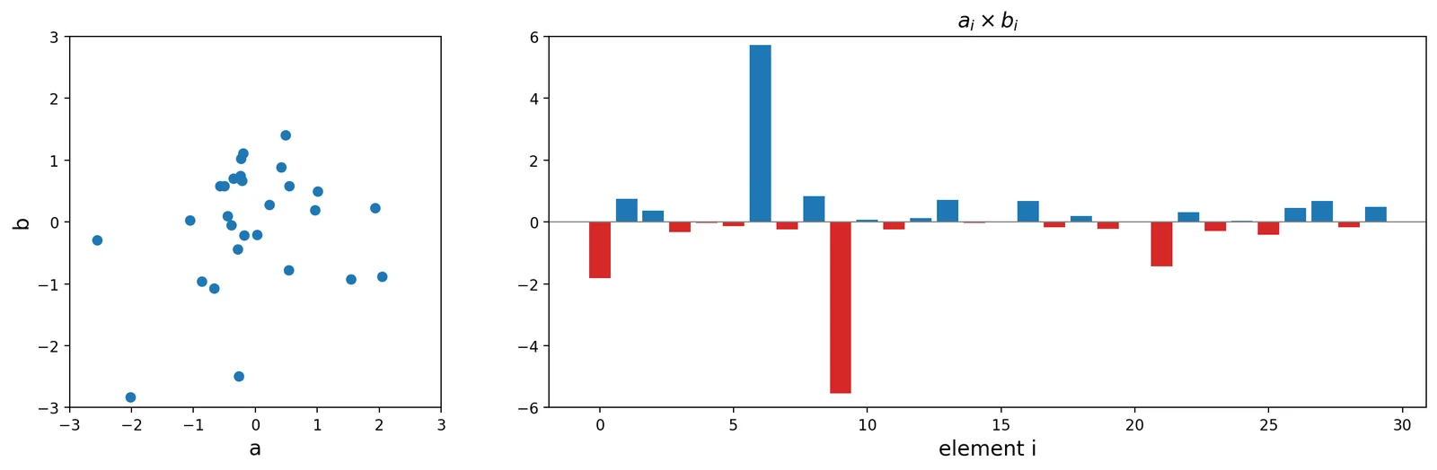
To understand convolution, we first need to familiarize ourselves with the dot product. The dot product is simply the sum of the elements of a vector weighted by the elements of another vector. This method is commonly used in signal processing, and also in statistics as a measure of similarity between two vectors. Finally, there is also a geometric interpretation which is a mapping between vectors (i.e., the product of the magnitudes of the two vectors scaled by the cosine of the angle between them). For a more in depth overview of the dot product and its relation to convolution, you can watch this optional video.Dot Product: 567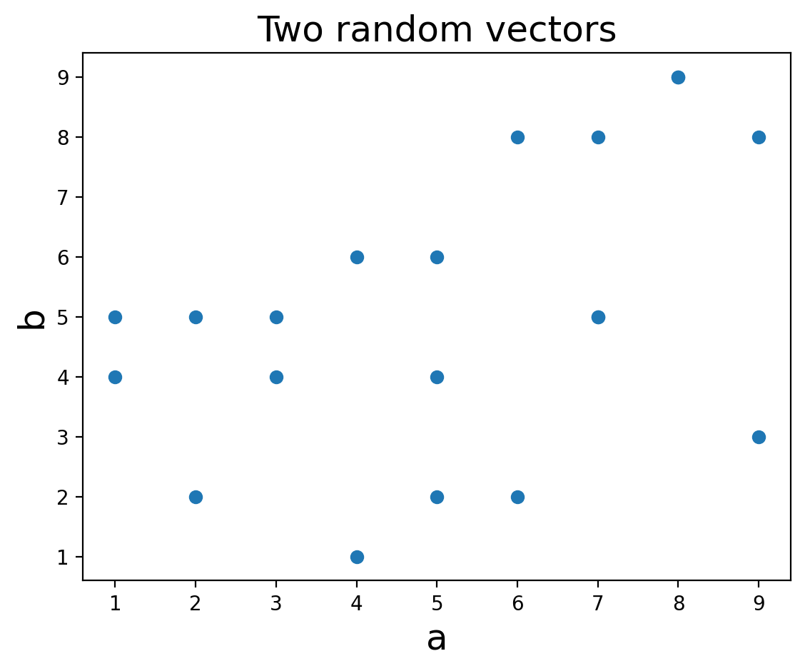
Convolution
Convolution in the time domain is an extension of the dot product in which the dot product is computed iteratively over time. One way to think about it is that one signal weights each time point of the other signal and then slides forward over time. Let's call the timeseries variable signal and the other vector the kernel. To gain an intuition of how convolution works, let's play with some data. First, let's create a time series of spikes. Then let's convolve this signal with a boxcar kernel.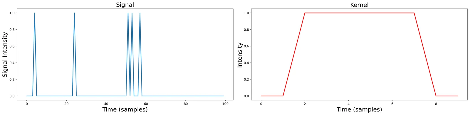
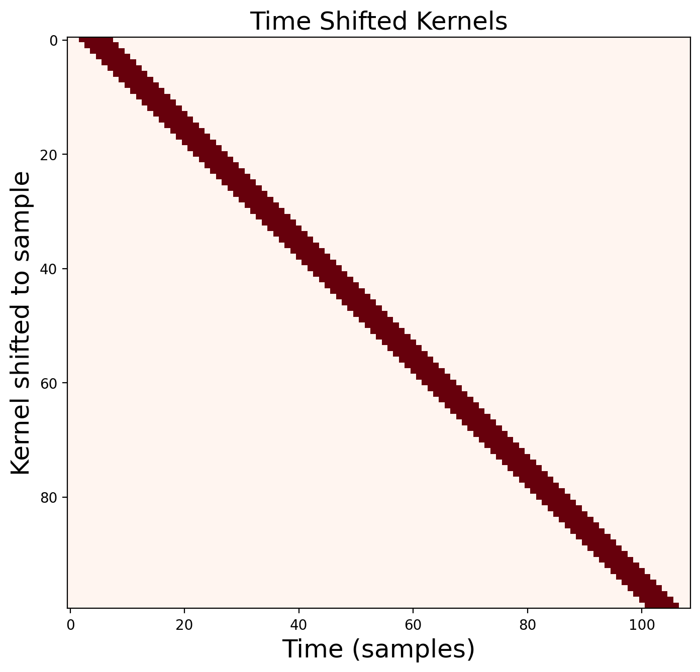
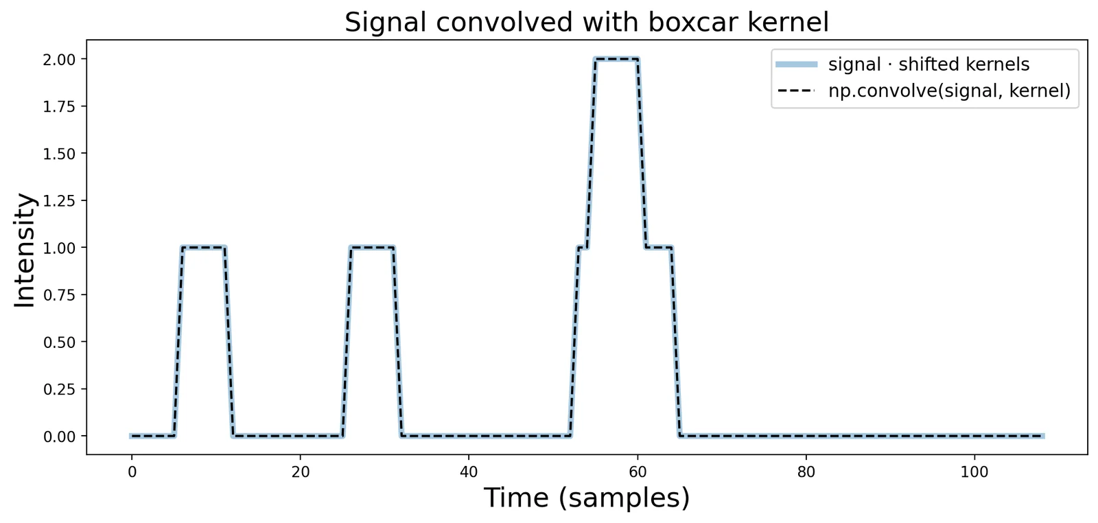 After convolution, each spike has become the shape of the kernel.
 np.convolve (dashed) does exactly this matrix multiplication for us.
Signal: 100, Kernel: 10, Convolved: 109 samples (the kernel hangs off the end).Step Through Convolution
Use the slider to step through the convolution one timepoint at a time. Watch the kernel (red) slide across the signal and see the output build up.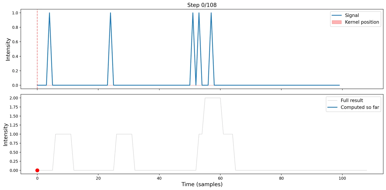
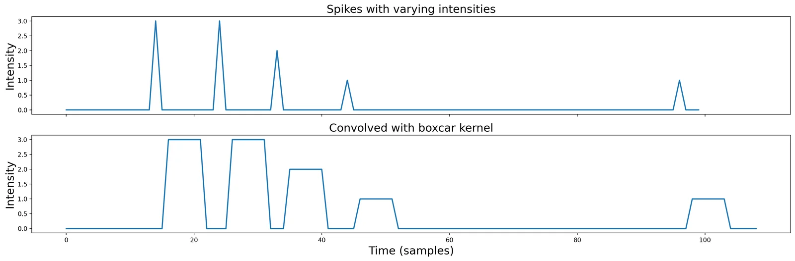
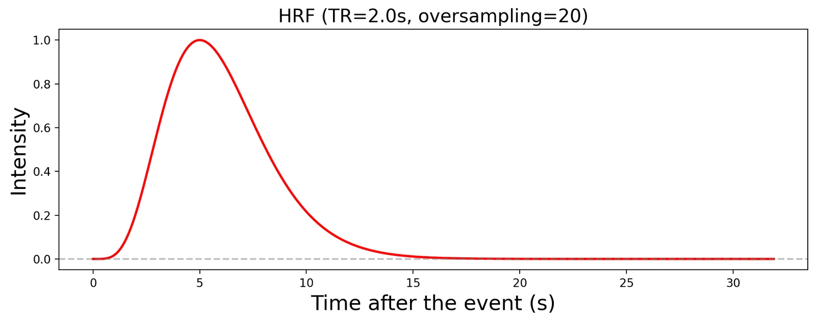
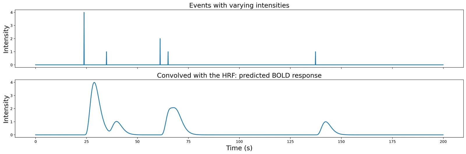
Oscillations
Ok, now let’s move on to studying time-varying signals that have the shape of oscillating waves. Let’s watch a short video by Mike X Cohen to get some more background on sine waves. Don’t worry too much about the matlab code as we will work through similar Python examples in this notebook.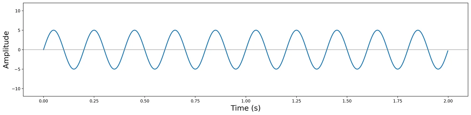
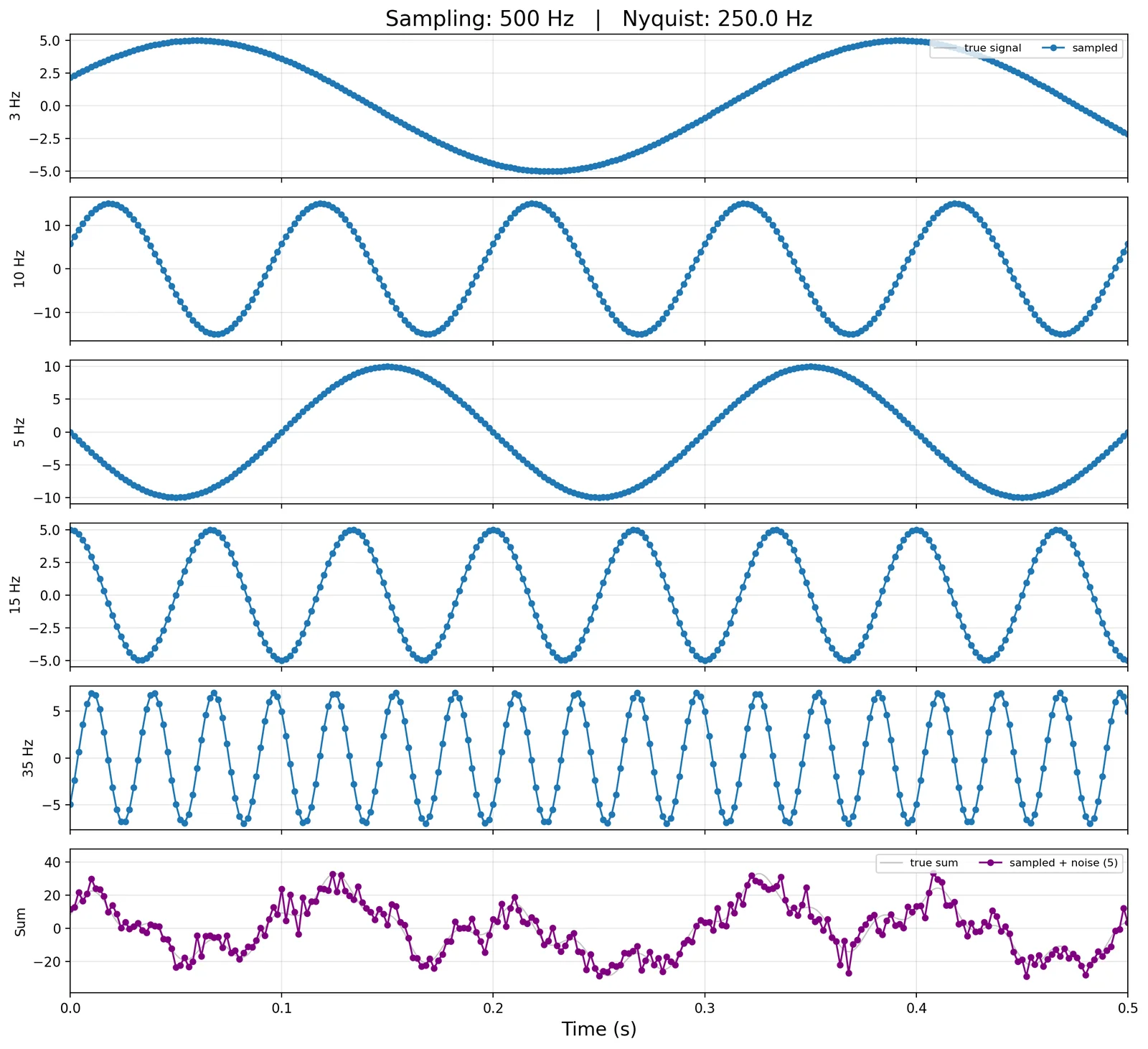
Aliasing at fMRI sampling rates
This matters for fMRI. We sample the brain once per TR (repetition time), so the sampling frequency is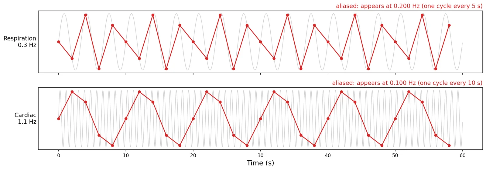
Time & Frequency Domains
We have seen above how to represent signals in the time domain. However, these signals can also be represented in the frequency domain. Let’s get started by watching a short video by Mike X Cohen to get an overview of how a signal can be represented in both of these different domains.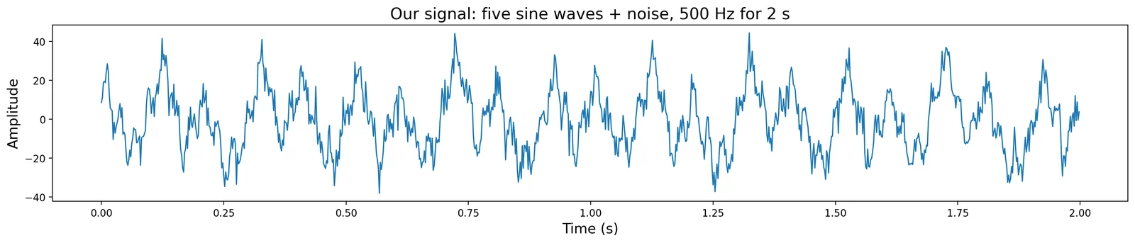
Frequency Domain
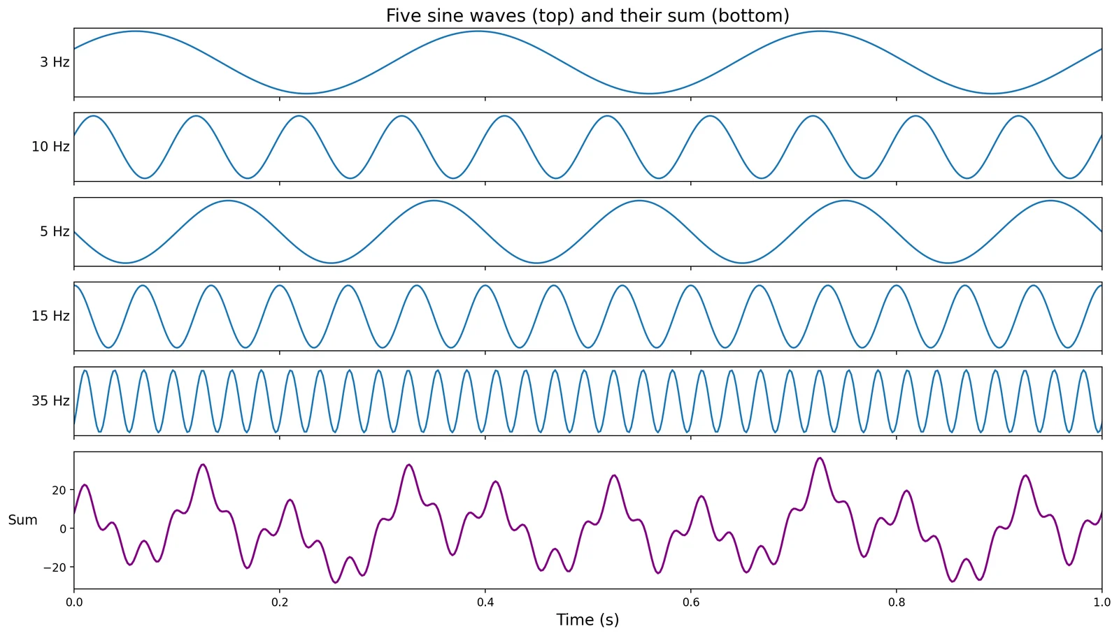
In the previous example, we generated a complex signal composed of multiple sine waves oscillating at different frequencies. Typically in data analysis, we only observe the signal and are trying to uncover the generative processes that gave rise to the signal. In this section, we will introduce the frequency domain and how we can identify if there are any frequencies oscillating at a consistent frequency in our signal using the fourier transform. The fourier transform convolves different frequencies of sine waves with our data to identify oscillatory components. One important assumption: stationarity — the generative processes don't vary over time. See this video or a more in depth discussion on stationarity. In practice, this assumption is rarely true. Often it can be useful to use other techniques such as wavelets to look at time x frequency representations. We will not be covering wavelets here, but see this series of videos for more information.Discrete Time Fourier Transform
We will gain an intution of how the fourier transform works by building our own discrete time fourier transform. Let’s watch this short video about the fourier transform by Mike X Cohen. Don’t worry too much about the details of the discussion on the matlab code as we will be exploring these concepts in python below.Complex Sine Waves
You may have noticed that we are computing complex sine waves using thenp.exp function instead of the np.sin function.
np.real or the imaginary using np.imag.
We can visualize complex sine waves in three dimensions. For more information, watch this video. If you need a refresher on complex numbers, you may want to watch this video.
In this plot, we show this complex signal in 3 dimensions and also project on two dimensional planes to show that the real and imaginary create a unit circle, and are phase offset by 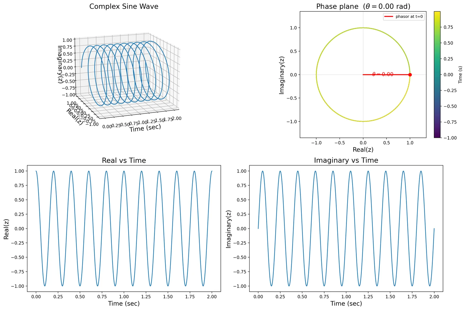
Create a filter bank
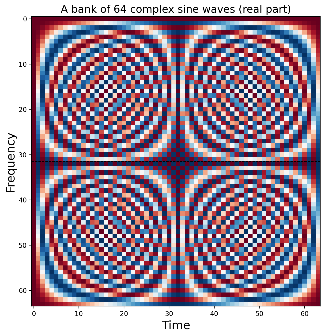
Ok, now let’s create a bank of n-1 linearly spaced complex sine waves and the plot first 5 waves to see their frequencies. Remember the first basis function is zero frequency (DC) component and reflects the mean offset over the entire signal.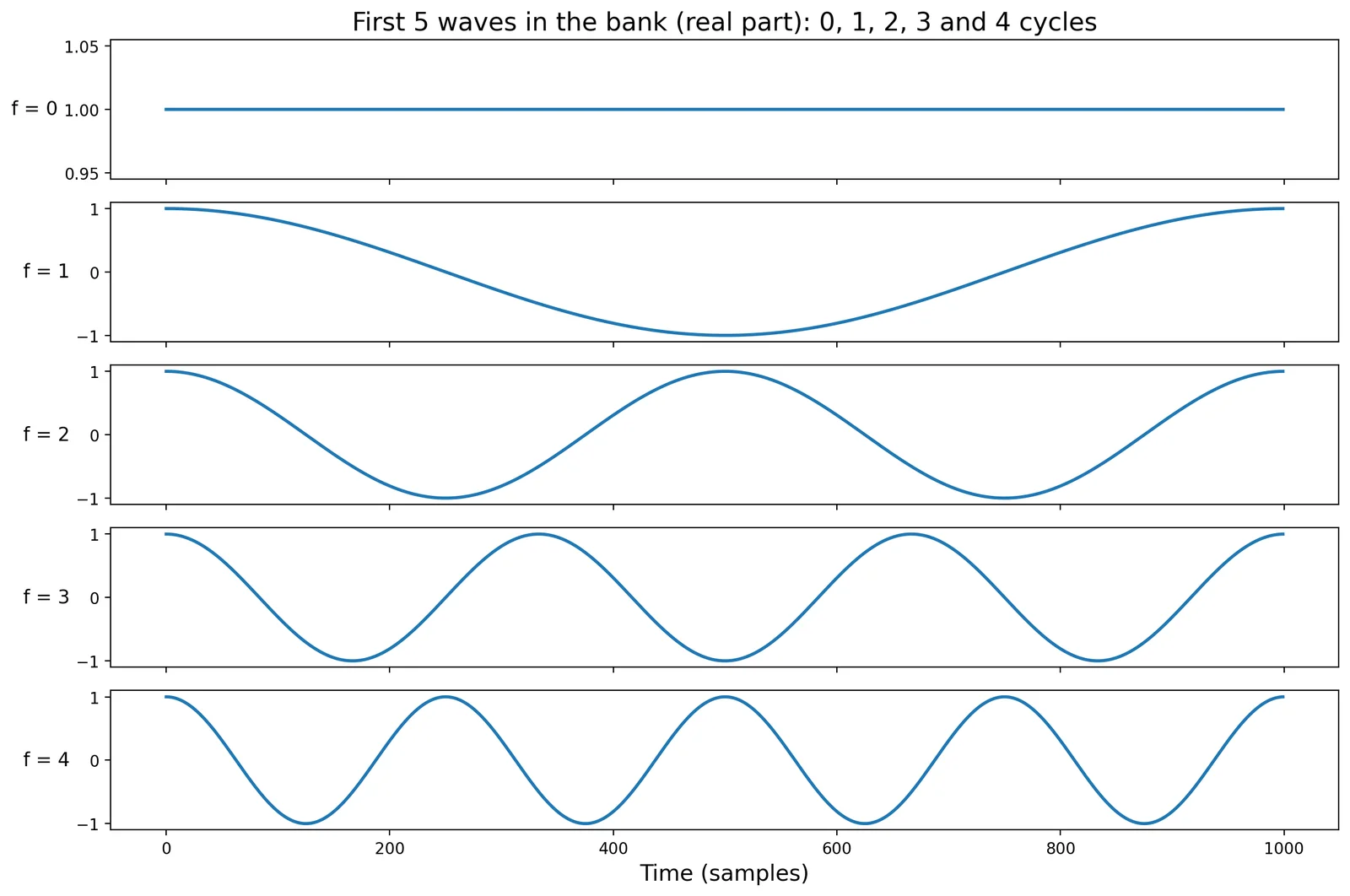
Estimate Fourier Coefficients
Now let’s take the dot product of each of the sine wave basis set with our signal to get the fourier coefficients. We can scale the coefficients to be more interpretable by dividing by the number of time points and multiplying by 2. Watch this video if you’re interested in a more detailed explanation. Basically, this only needs to be done if you want the amplitude to be in the same units as the original data. In practice, this scaling factor will not change your interpretation of the spectrum.Recall: 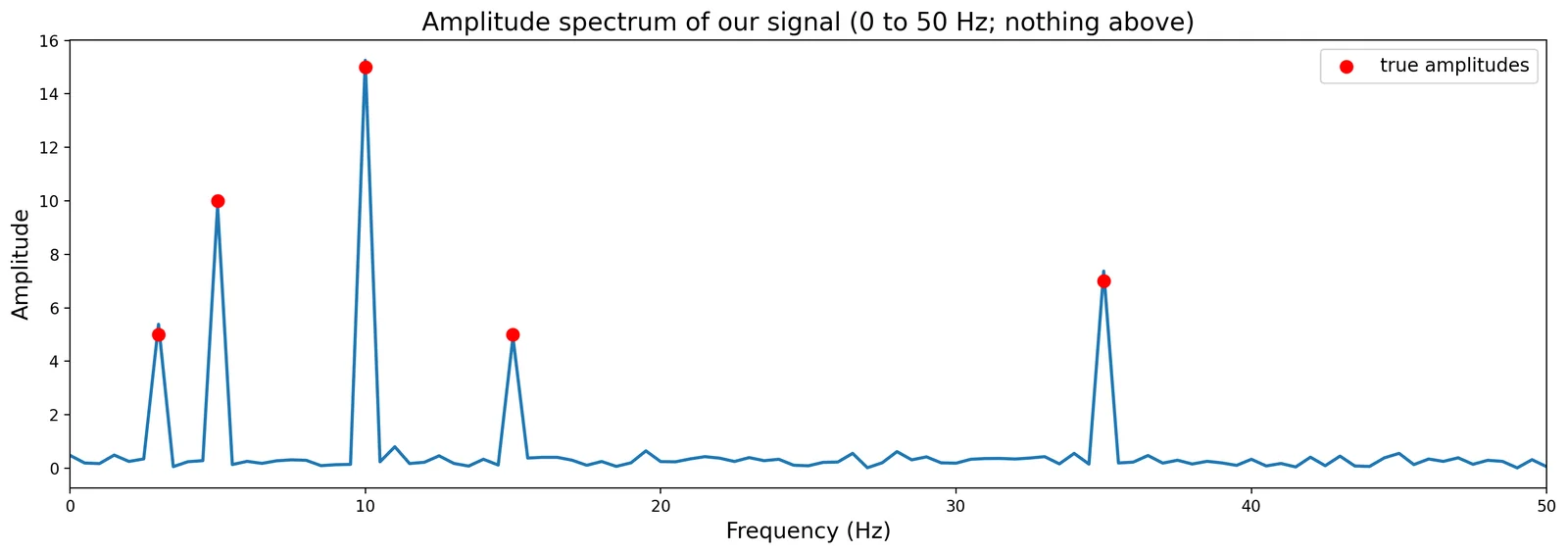 Each coefficient belongs to one frequency: coefficient
 ||(k||) is ||(k||) cycles per recording, so with 2 s of data it sits at ||(k / 2||) Hz. In practice you'd use ||(O(n \log n)||) operations instead of ||(O(n^2)||) . That's the fast Fourier transform.
freq = [3, 10, 5, 15, 35], amplitude = [5, 15, 10, 5, 7]. Each peak lands on (or, because of the noise, very near) its true amplitude, shown as red dots. The small bumps everywhere else are the noise.Each coefficient belongs to one frequency: coefficient np.fft.fft, which computes exactly these coefficients (np.allclose → True) much faster: Let's learn a few more important details about the DFT:
Inverse Fourier Transform
The fourier transform allows you to represent a time series in the frequency domain. This is a lossless operation, meaning that no information in the original signal is lost by the transform. This means that we can reconstruct the original signal by inverting the operation. Thus, we can create a time series with only the frequency domain information using the inverse fourier transform. Watch this video if you would like a more in depth explanation.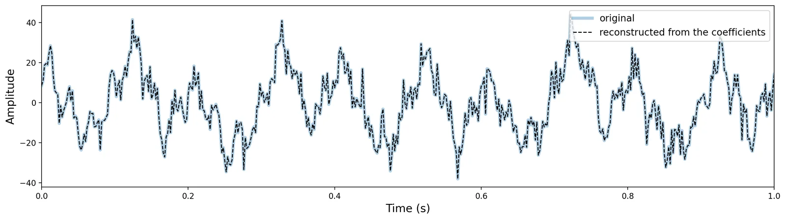 Largest difference from the original: 9.4e-12, i.e. rounding error.
Phase Spectrum
Each Fourier coefficient is a complex number, so it carries two things: its size (the amplitude, plotted above) and its angle (the phase). The phase says where in its cycle each wave is at time zero. Phase is only meaningful at frequencies where there is a real oscillation; elsewhere it is just the phase of the noise. So below we read off the phase at our five frequencies and compare it to the phases we used to build the signal. The FFT measures phase relative to a cosine, and a sine is a cosine shifted by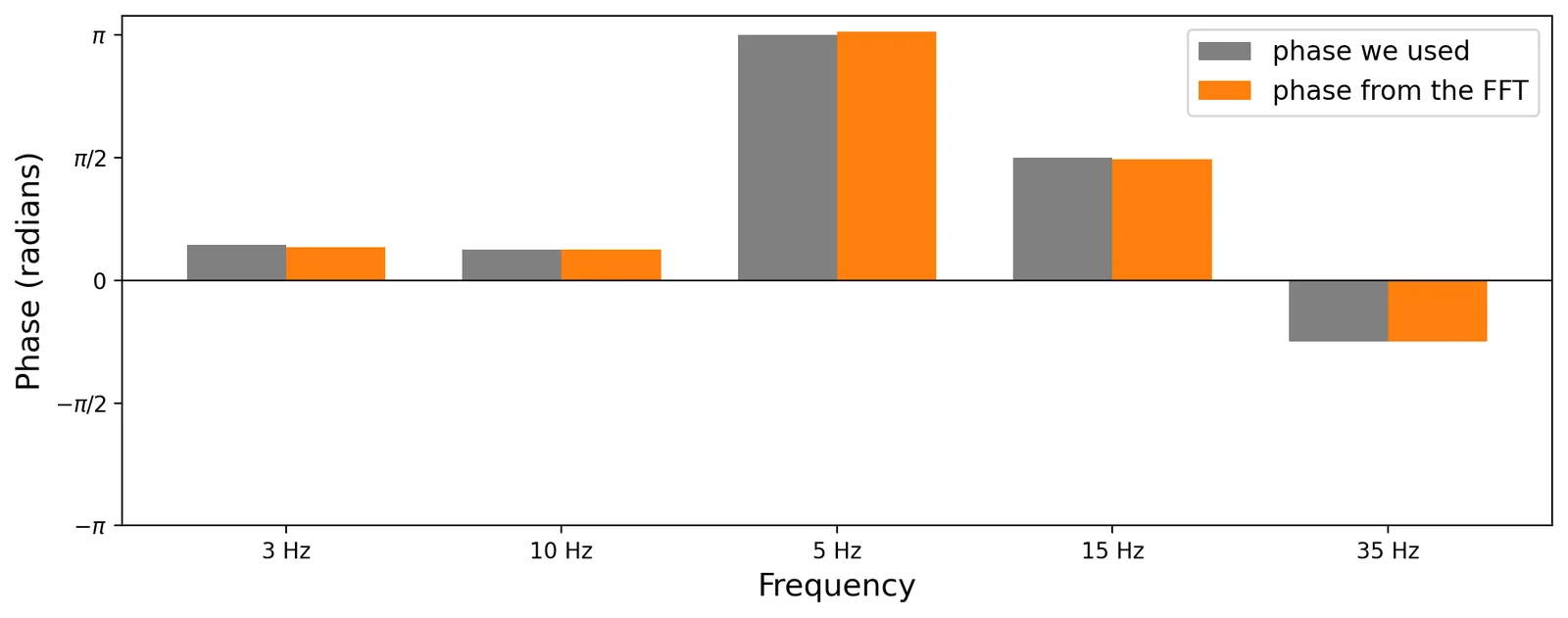
Convolution Theorem
Convolution in the time domain is the same as multiplication in the frequency domain. This means that time domain convolution computations can be performed much more efficiently in the frequency domain via simple multiplication. (The opposite is also true: multiplication in the time domain is the same as convolution in the frequency domain.) Watch this video for an overview of the convolution theorem and convolution in the frequency domain. Below, the top row convolves our signal with a short smoothing kernel in time. The bottom row shows the same three things in the frequency domain: the signal's spectrum, times the kernel's spectrum, gives the spectrum of the result.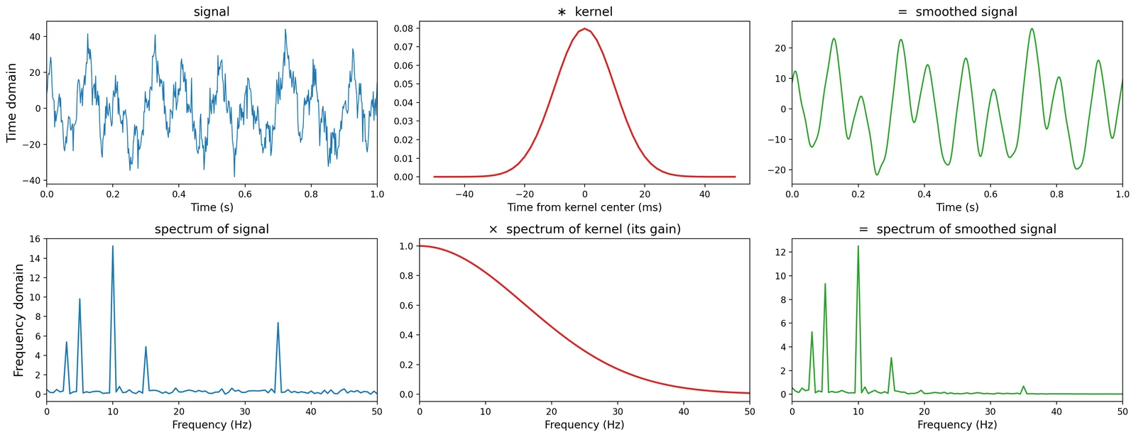
Filters
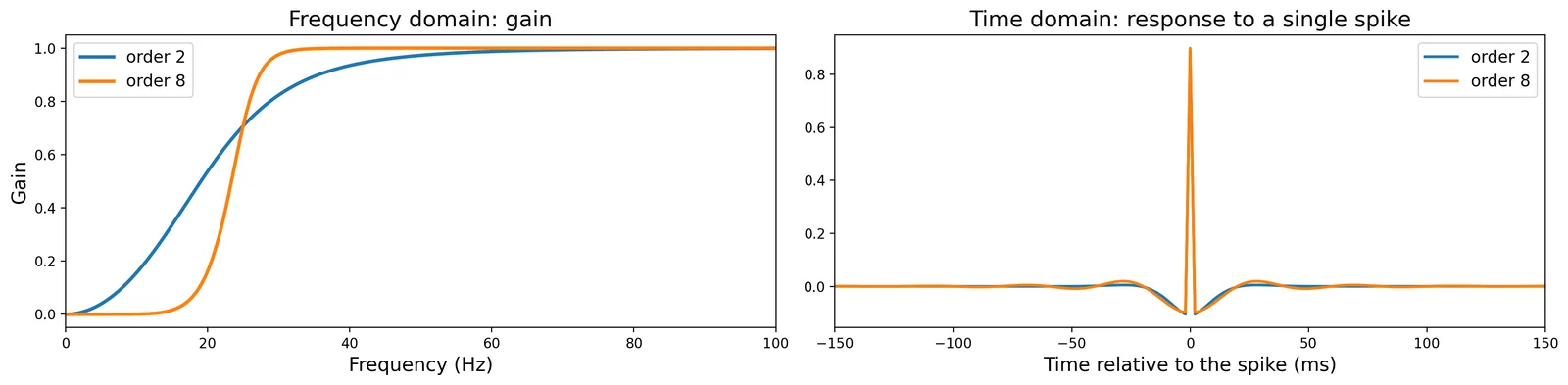
A filter changes how much of each frequency survives. It can be described in two equivalent ways:- In the frequency domain, by its gain: a number for every frequency, from 1 (keep it) to 0 (remove it).
- In the time domain, by its kernel, also called its impulse response: the output you get when you feed the filter a single spike.
- ripple in the pass-band
- attenuation in the stop-band
- steepness of roll-off
- filter order (i.e., length for FIR filters)
- time-domain ringing
Two ways to apply the same filter
Let's apply one low-pass filter both ways. The signal has two components, a slow 5 Hz wave and a fast 35 Hz wave, and the filter should keep everything below 15 Hz. We'll use a simple FIR filter fromscipy.signal.firwin, whose kernel is just a list of 101 weights.
Way 1: in the time domain, convolve with the kernel
This is exactly the convolution from the start of this chapter. Slide the kernel along the signal and take a dot product at every time point. The kernel is a smooth bump, so each output sample is a weighted average of its neighbors. Averaging over ~100 ms smooths away the fast 35 Hz wiggles but barely touches the slow 5 Hz wave.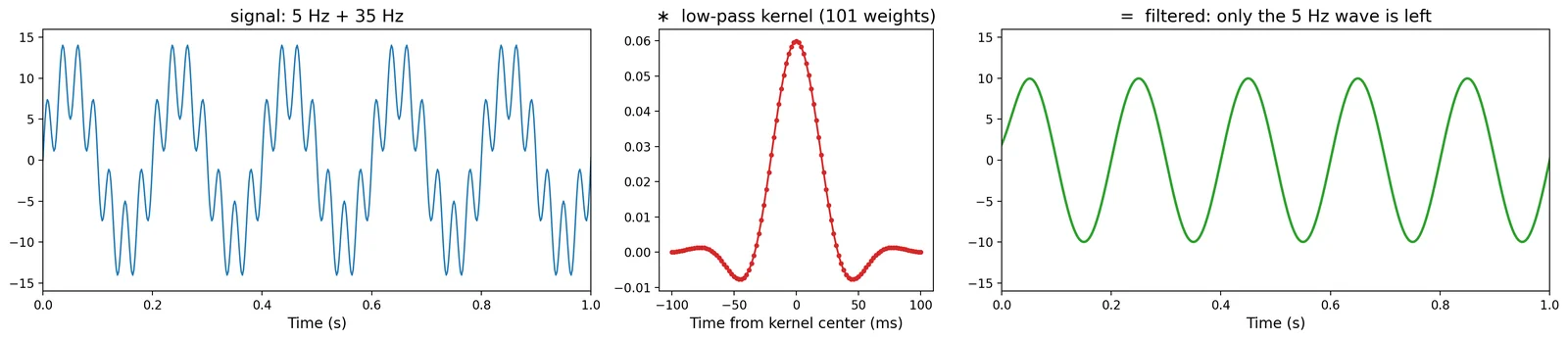
Way 2: in the frequency domain, multiply by the gain
- Take the FFT of the signal. Remember that the FFT returns positive and negative frequencies: the second half of the array is a mirror image of the first. The plots below show only the positive half.
- Build the filter's gain at every FFT frequency, the negative ones included, so the mirror image stays intact. Here we take the FFT of the kernel, padded to the length of the signal, which takes care of both halves. Because the kernel is symmetric, its gain is real-valued: about 1 below 15 Hz and about 0 above.
- Multiply the two, frequency by frequency.
- Take the inverse FFT to get back to time. The result should be real;
.realdrops the leftover rounding error.
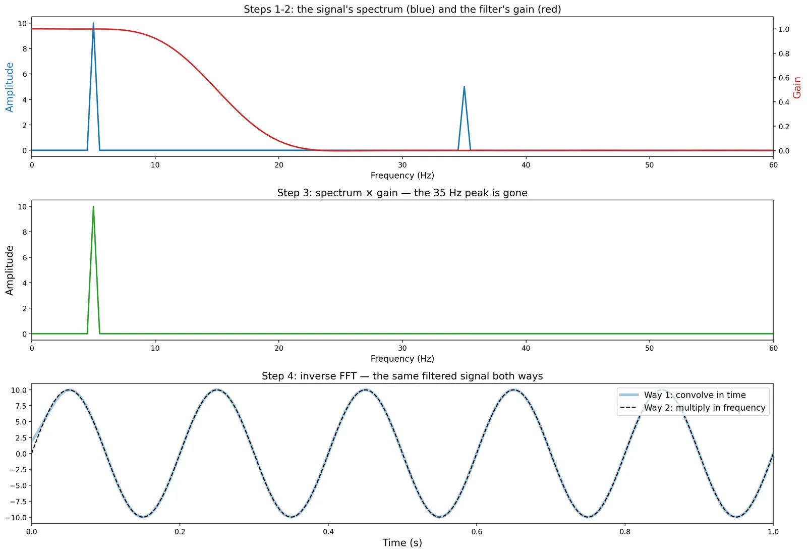 Away from the edges, the two results differ by at most 5.3e-15, i.e. only by rounding error.
Which one is used in practice?
Both, and you'll meet each:- Frequency domain: you see exactly what the filter does to every frequency, and for long signals the FFT makes it fast. Watch the edges, though: the FFT treats the signal as if it wraps around in a loop, so the end leaks into the beginning.
- Time domain: works on a stream, one sample at a time. Real-time audio does this. The equalizer later in this chapter filters your music in the time domain, with small IIR filters running sample by sample, while its gray spectrum display is an FFT.
scipy.signal.filtfilt, which we use for the Butterworth filters below, is also a time-domain method. Butterworth filters are IIR, so instead of convolving with a fixed kernel, each output sample is computed from recent inputs and recent outputs.filtfiltruns the filter forward and then backward, which cancels the time shift a one-way filter would add.
Two easy mistakes in the frequency domain
- Forgetting the negative frequencies. If you set the gain at +35 Hz to 0 but not at −35 Hz, the spectrum is no longer mirror-symmetric, and the inverse FFT comes back complex instead of real.
- A brick-wall gain. Jumping straight from 1 to 0 at the cutoff is the sharpest filter possible in frequency, so by the frequency × time trade-off it rings in time. You can see this around sharp edges, like the onsets of a block design.
Mistake 1: zeroing only the positive frequencies above 15 Hz leaves an imaginary part as large as 2.50 after the inverse FFT. Zero the negative ones too (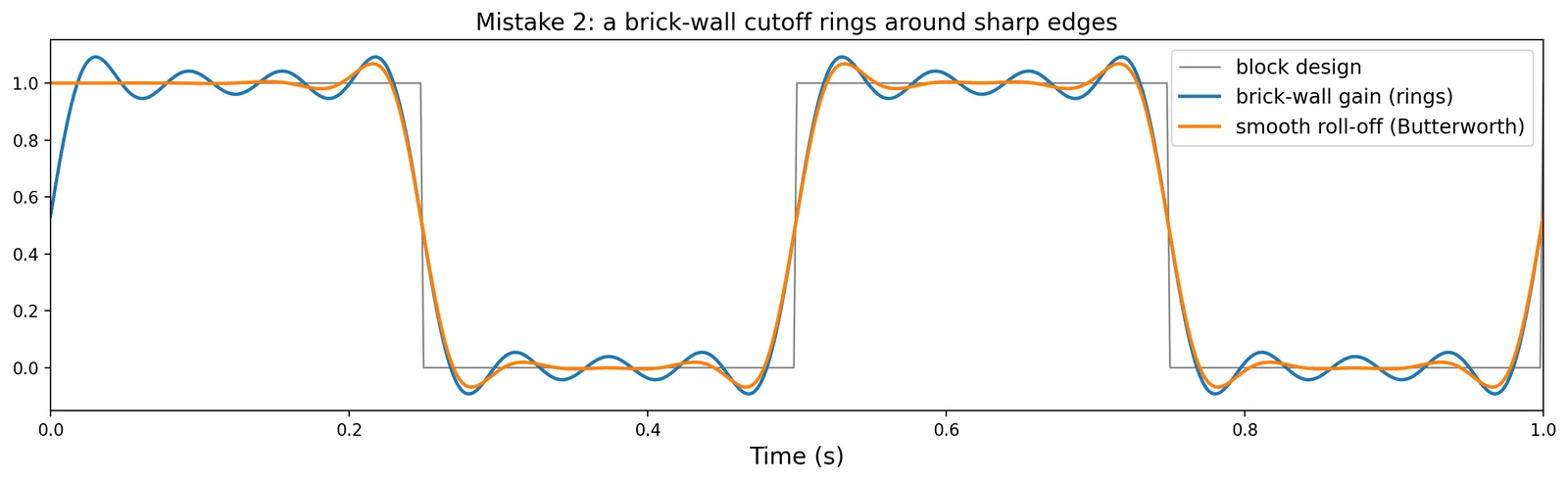
np.abs(freqs) > 15) and it drops to rounding error.Four common filters
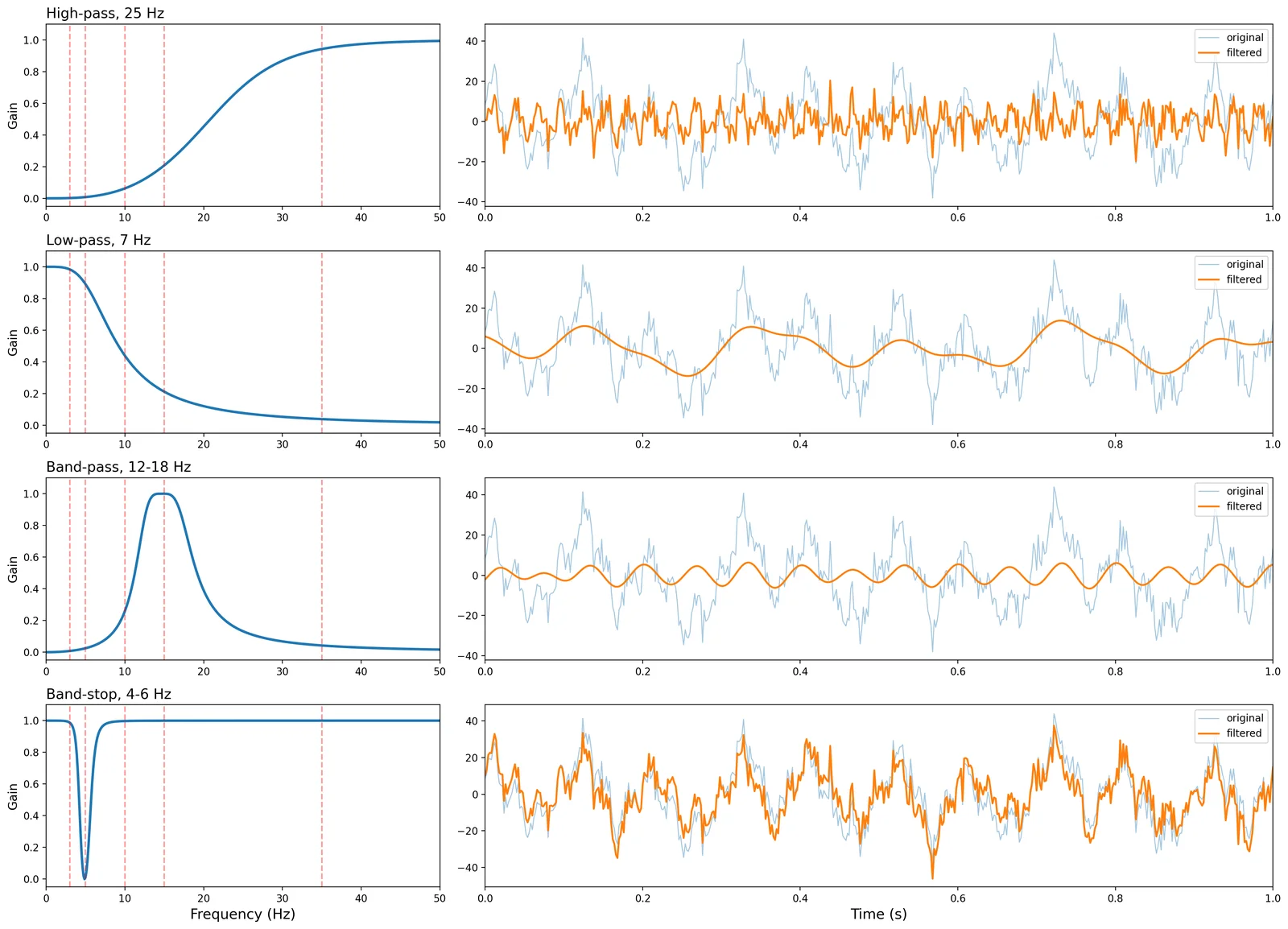
From here on we'll use IIR Butterworth filters, applied in the time domain withfiltfilt. There are four basic types, named for what they let through:
- High-pass keeps frequencies above a cutoff and removes slow ones (like scanner drift).
- Low-pass keeps frequencies below a cutoff and removes fast ones.
- Band-pass keeps only a range of frequencies. A Morlet wavelet, for example, is a band-pass filter centered on one frequency.
- Band-stop removes a range of frequencies and keeps everything else.
filtfilt runs the filter forward and then backward over the whole recording, so its response is symmetric around the spike. That's what keeps it from shifting the signal in time, and it's possible because we filter a recording after the fact, not a live stream.
Interactive Filter Explorer
Explore all filter types interactively: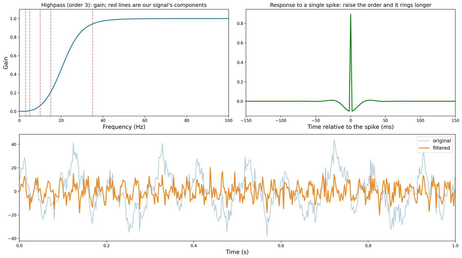
High-pass filtering fMRI data
The most common filter in fMRI preprocessing is a high-pass filter. It removes slow scanner drift, which otherwise dwarfs the effects we care about. The simulated voxel below has a block design (20 s on, 20 s off, so the task repeats every 40 s, or 0.025 Hz) sampled at TR = 2 s, plus slow drift and noise. The cutoff is usually written as a period, in seconds per cycle, rather than a frequency. Use the slider to choose it. Everything slower than that period is removed (the red band in the spectrum). What happens when the cutoff period is shorter than the 40 s task cycle?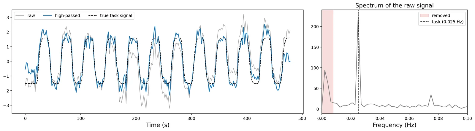
Hearing filters
Filters are easier to understand when you can hear them. Music is a mixture of many frequencies at once: the kick drum and bass live below ~250 Hz, voices and most instruments between ~250 Hz and 4 kHz, and the hiss of cymbals and the "air" of a recording above ~4 kHz. Drop any song (mp3, wav, …) onto the player below. It loops, and every sound passes through a bank of filters before it reaches your speakers. Each handle sets the gain at one frequency, from 1 (pass it through untouched) to 0 (remove it), with low frequencies on the left — exactly like the filter plots above. The dark curve is the filter's actual frequency response, and the gray shading is the spectrum of what you are hearing right now. Your file never leaves your browser.- Click Low-pass. Which instruments disappear, and which survive? Now drag the 500 Hz and 1k handles back up — how does moving the cutoff change the sound?
- Click High-pass. What happens to the bass and drums? Why does the song sound "thin"?
- Click Band-pass, which keeps only ~500 Hz–1 kHz. Why does it sound like an old telephone or AM radio?
- Click Band-stop and listen to what is missing. Compare the gray spectrum to the one you see with Flat.
- Look at the curve between handles. Even a sharp step on the sliders becomes a smooth roll-off — a real filter can't jump from 1 to 0 at a single frequency. How does that relate to the filter order you explored above?
Exercises
Exercise 1: Create a simulated time series with 7 different frequencies with noise
Ellipsis
Exercise 2: Show that you can identify each signal using a FFT
Ellipsis
Exercise 3: Remove one frequency with a bandstop filter
Ellipsis
Exercise 4: Remove frequency with a bandstop filter in the frequency domain and reconstruct the signal in the time domain with the frequency removed and compare it to the original
Ellipsis
Graded assignment
The graded version of these exercises is the Signal Processing assignment at the end of this page, which opens in a drawer from the Assignment button in the header. Open it from that page (in molab or by download), sign in with your Dartmouth account inside the notebook, and submit each question when you are ready.Assignment: Signal Processing
- Setup
- Q1. Simulate a time series with 7 frequencies plus noise
- Q2. Identify each frequency with an FFT
- Q3. Remove one frequency with a bandstop filter
- Q4. Remove the same frequency in the frequency domain
- Q5. Interpretation
Open in molab
Opens in a drawer at the bottom of the page, so you can keep reading while you work. Autosaves in this browser.